Part I: Sentiment analysis on Yelp reviews for a retail chain, the case of Starbucks.
Understand this project in one pic
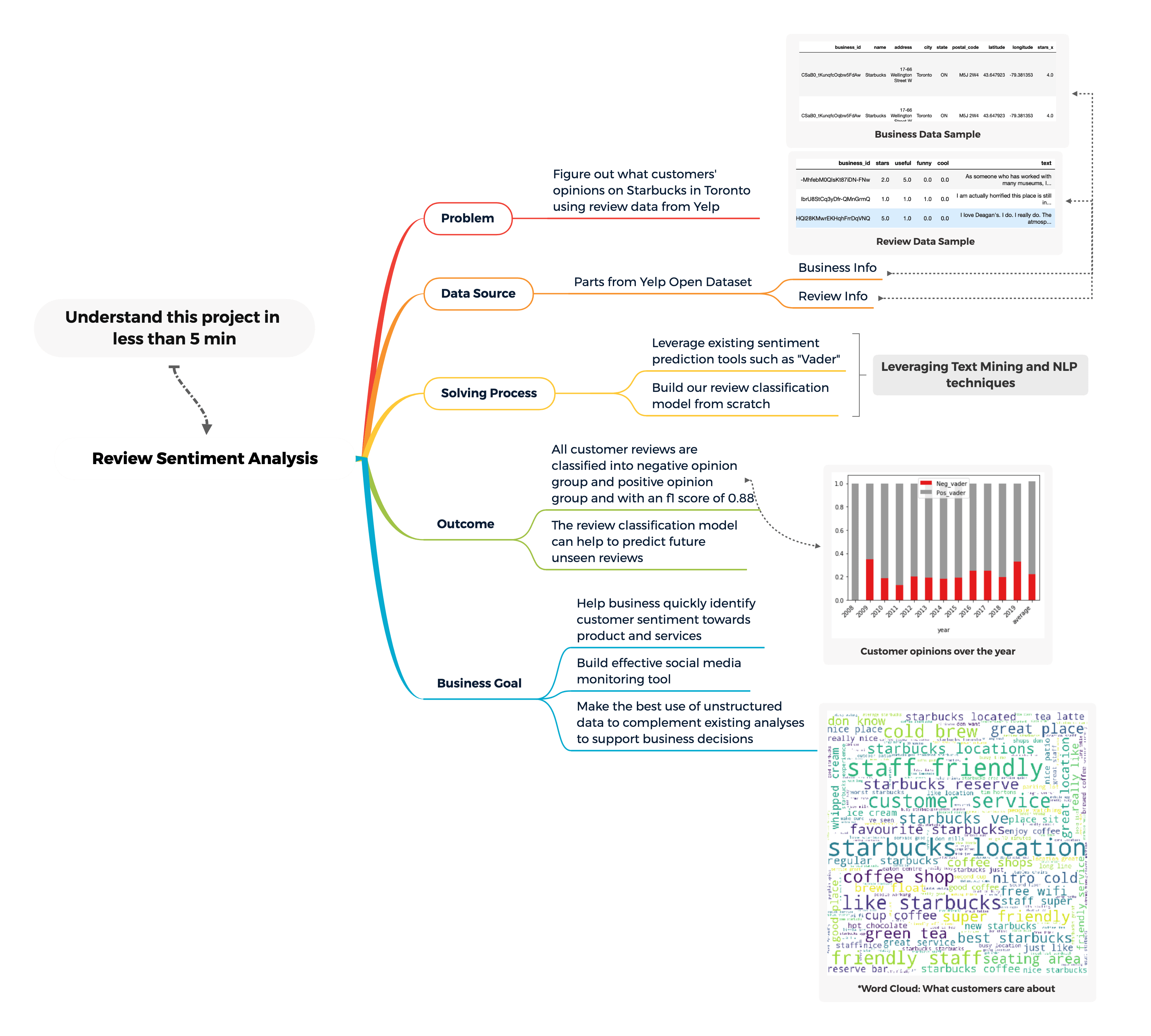
Overview of the project:
Social media monitoring is one powerful way to help businesses quickly assess their customer's opinion toward them. Imagining that you work for a retail chain as a data scientist, and the management expects you to update the customer experience and satisfaction with the brand periodically, and to achieve these, you are most likely evaluating internal data such as direct survey results, changes in sales quantity, different marketing campaigns' responses and possibly external data including third-party survey results and reviews from different websites and platforms.
The key thing here is, as data scientists, we want to leverage the right skills and tools to help decision-makers to discover whether our products, services, and implemented strategies are aligned with the current market demand. If not, how can the business cope with shifts in demand with help from data analysis and data science?
If we were to compare different data sources for evaluating customer satisfaction. We can certainly use a direct approach by issuing surveys to our customers both in-person at the store or electronically via emails to ask them using a set of questions, tailored by our marketing teams and product teams. Besides, we can also rely on third-party market research organizations to investigate and provide aggregated results to understand the business's current position in the market. Both approaches can help us determine customer satisfaction but neither one provides an adaptable solution to a constantly changing topic like customer experience. Both approaches are resource costly and static and we want to actively monitor opinions and mentions made by our customers. Hence, one of the main goals for this project is to build an automated sentiment analysis procedure using machine learning techniques to help businesses discover if their customers are happy or unhappy at any given time.
Moreover, since the data we got comes with labels thus we are also interested in building a review prediction model to accurately classify unseen reviews to either good or bad which in result, increase the efficiency of social media monitoring.
Last but not least, we want to build topic models and perform in-depth analyses on the negative reviews made toward our brand or products and see if we can give any recommendations to the management.
Project Breakdown:
This project is divided into the following two parts:
Part I: a complete exploratory data analysis of the given dataset, sentiment analysis on all reviews made available, and a classification model to predict whether a review is positive or negative using given training labels.
Part II: topic modelling on the recent three years' reviews and isolates negative reviews made to the business so we can work on the improvements.
Tools used:
All analyses and model buildings are achieved using Python and its associated packages such as Numpy, Pandas, Scikit-Learn, Gensim and NLTK…etc.
Data Availability:
I chose the famous Yelp Open Dataset for this NLP project, and the dataset is managed and updated by Yelp yearly to support personal, educational and academic uses. This dataset contains 5 separate JSON file with Yelp's business data, review data, and user data.
Another important reason on why to use this dataset is because Yelp is one of the main platforms which general public use to leave their opinions at about the businesses. The actions of leaving reviews by the customer are completely voluntary, thus comparing to official survey results, it tends to provide additional unknown information that is valuable to the businesses.
Objectives and Methodologies:
Part I: Detect our customers' opinions whether it is positive or negative through sentiment analysis. Sentiment Analysis, by definition, is "the interpretation and classification of emotions (positive, negative and neutral) within text data using text analysis techniques".
Two existing sentiment analysis tools are used in this part of the project, Vader, a lexicon and rule-based tool specifically attuned for social sentiment analysis, and also Textblob, a Python library with simple API for many natural language processing tasks including sentiment analysis.
The review prediction model is built using a tree-based bootstrap aggregation algorithm called "Random Forest".
Part II : Topic modelling on recent year's customer reviews to understand shifts in market demand and to detect issues with current strategies or products…etc. Topic modelling is an unsupervised learning technique used to study underlying topics in a collection of documents. The algorithm I chose in this project is called "Latent Dirichlet Allocation" also known as "LDA", and it utilizes a probabilistic approach to find "hidden" topics in our customer's reviews or complaints.
Part 1 Begin: Data Understanding and Exploration:
Loading and selecting data
The original dataset contains 5 separate data files in JSON format. After some initial explorations and readings from the official documentation, I chose to use "Business.json" and "Review.json" files only.
The business data contains information about the businesses such as names, unique business ids, and locations etc. The review data contains information such as stars ratings, review texts, and time stamp etc, and it can be merged with the prior business data through unique business ids.
These two files are first transformed to CSV format using a customized function and then they were loaded into two separate Pandas data frames.
This is what business data looks like: (60 columns in total, 10 shown)

This is what review data looks like : (9 columns in total, 9 shown)
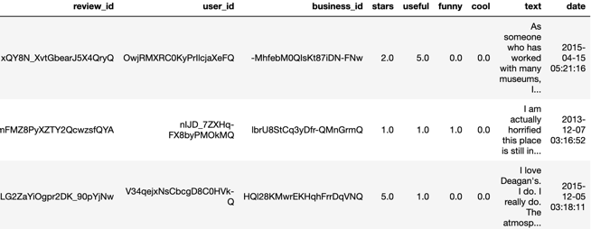
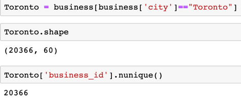
For demonstration purpose, I want to filter data to include only "Toronto" wise data and to include only "Starbucks" reviews.
Step 1: (there are 20366 unique businesses in Toronto)
Step 2: (merge two tables, and we get 600584 reviews in total for businesses in Toronto)

Step 3: (Include "Starbucks" only stores, and we have 1814 reviews in total)
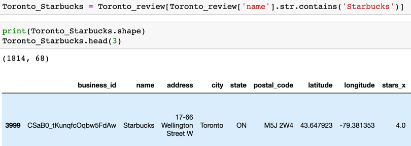
The fact that there aren't that many reviews in our selected data is a bit of a surprise considering its giant customer base in Canada. Maybe, it is because the vast majority of its customers are only stopping by to grab a coffee to go and they are not spending too much time inside the store. Alternatively, customers may choose to leave their reviews elsewhere such as website like Google.
More about the data.
1814 total reviews are made to 161 unique Starbucks stores. These 161 stores are not the total number of stores in Toronto and are only those who ever received any reviews on Yelp.

The minimum number of reviews received by a store is 3, and the maximum is 60.

Reviews are made spread across 12 years (later I will break down it into years)

Filter the entire dataset based on the columns of interests for Sentiment Analysis

Notice that I selected a column called "stars_binary", and renamed it to "true_sent". Basically, "stars_binary" is "stars" column transformed into a binary format which represents the individual rating of customer experience about their recent interaction with the store.
It can be viewed as a high-level representation of customer reviews. Hence, I used this column as the true sentiment labels for this project. Originally, it has 5 ratings from a scale of 1 to 5, and from 1 the least satisfied to 5 the most satisfied. Now it is 0s which consists of scale from 1-3 and 1s which consists of scale from 4-5.


We can see that there are 1396 positive reviews and 418 negative reviews so about 77% of positive reviews and 23% of negative reviews. I will come back for this later.
Split the data by year (12 years in total), and find more insights.

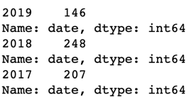
Now the entire data is divided into each year's data, and the first thing we found is on average there are 151 reviews each year.

However, when we look at the recent three years of data, we realized the number of reviews left on Yelp regarding Starbucks decreased by more than 40% from the year 2018 to the year 2019. The number of reviews in 2019 which is 146 is below the historical average of 152.
Part I Continues: Sentiment Analysis:
"Sentiment analysis is the interpretation and classification of emotions (positive, negative and neutral) within text data using text analysis techniques. Sentiment analysis allows businesses to identify customer sentiment toward products, brands or services in online conversations and feedback" – Monkey Learn.
There are several different ways to perform a sentiment analysis task, such as a rule-based approach or an automatic approach or a hybrid of two. For more in-depth and detailed explanations about sentiment analysis, please visit "https://monkeylearn.com/sentimentanalysis/", "https://en.wikipedia.org/wiki/Sentiment\_analysis".
Vader Sentiment Prediction:
The first method I chose for this task belongs to the rule-based approach, and it is an open-sourced tool accessible from NLTK named "Vader" or the "Valence Aware Dictionary and sEntiment Reasoner".
How Vader works in simple terms:
It internally utilizes a lexicon of sentiment-related words. When you feed Vader a piece of text to analyze, it will check to see if any words in the text are presented in this lexicon. Not only it will tell you whether this piece of text is negative or positive but also tell you the magnitude of how positive and negative this text is.
Vader is specifically designed to incorporate "special cases" where cannot be seen in formal and traditional language settings such as "emojis" and "slangs" that appear most in social media texts. There are many more advantages of using Vader for sentiment analysis such as its ability to handle the use of contractions as negations (e.g. wasn't very good) or use of punctuations to signal increased sentiment intensity (e.g. "Terrible!!!"). The best part of using a rule-based model is that it does not require any training data, polarities are determined by a pre-built, gold-standard sentiment lexicon.
Let's move our sights to the working details:

It is very easy to implement a Vader model. All I did above was to first isolate the text that we want to train our model on then build an analyzer using "SentimentIntensityAnalyzer". Lastly, calling a predict to our text using the analyzer built.
Check the result:

Vader model produces 4 different scores: "negative", "neutral", "positive" and "compound". The first three scores represent the proportion of text that falls in these three categories.
The "compound" score, according to the official documentation, is the most useful metric if you want a single unidimensional measure of the sentiment of a given sentence. How it is calculated is outside the scope of this project, but if you are interested, you can visit its official documentation. What we need to know is "compound" scores are between -1 (most extreme negative) and +1 (most extreme positive). Hence, to interpret the sentiment result for our first review:
It means that our first review was rated as 0% negative, 87.6% neutral and 12.4% positive, and based on its compound score of 0.8313, it is a very positive sentiment text.
Main assumption:
Recall previously we transformed "star", multiclass labels to "star_binary", binary labels. For consistency, we are only leveraging the "compound" score to evaluate the sentiment of the texts. We can manually set a threshold, so compound scores above this set threshold will be categorized as "positive" and below this threshold will be categorized as "negative".
We are setting the threshold to be equal to "0.05" as advice from the documentation.

We added the result back the data frame we used for model building and obtain the following:

We can easily spot that first three reviews have the same "vader_sent" prediction as to the "true_sent" labels. We can further calculate the accuracy of our Vader predictions:

Almost 83%, which is good and acceptable.
Textblob Sentiment Prediction:
As explained in the previous "Methodology and Object" section, "Textblob" is a Python library that offers a simple API to access its methods and functions to perform NLP tasks.
I am going to use the library's "sentiment" property to detect the underlying sentiment of the Starbucks reviews. Under the hood, Textblob's sentiment analyzer was pre-trained on a Naïve Bayes model using pre-classified movie reviews data, therefore you can use the analyzer directly to classify new text's polarity in positive and negative probabilities.
According to the official documentation: "The sentiment property returns a named tuple of the form Sentiment (polarity, subjectivity). A polarity score is a float number within the range [-1.0, 1.0]. The subjectivity is a float number within the range [0.0, 1.0] where 0.0 is very objective and 1.0 is very subjective".
Here, I only use the "polarity" score to determine whether a review is with positive or negative sentiment. However, this "subjectivity" detection feature is still very useful in other use cases.
Model Implementation:

Here, I also set the same threshold, so reviews with polarity score less than the threshold are considered to be negative and above is considered to be positive. We included the output in our data frame for modelling, and this is what we obtain:

Let's calculate this method's accuracy again:

We are getting 81% which is still acceptable but less accurate than the Vader model. So far, we have used two different approaches to predict the sentiment of the customers' reviews, and they both returning decent results. One major issue with these two models is they are not customized and specifically tuned for our dataset. Approaching the end of the project, we will build our machine learning models to predict the sentiment of these reviews and hoping to receive better results than the prior two models.
Post Sentiment Prediction Insights:
What else we can discover with the results from previous sentiment analyses?
First of all, we extract the "year" feature from the data.

Insight 1: We create a comparison table that consists of the results from two sentiment analysis models and we group by the results by year. The results are normalized to the relative frequencies of the unique values. Also, we calculated the overall average for each model's positive and negative result.
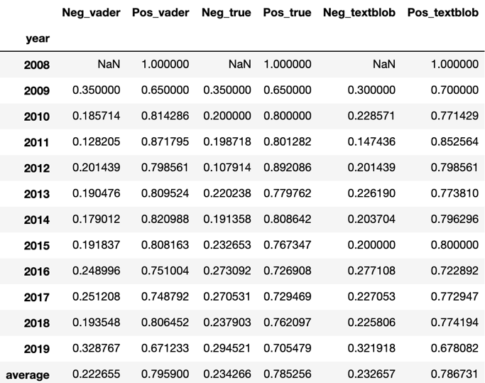
If we just look at the last row of this table, the first two columns are representing average Vader sentiment results over time. So, on average, 22.3% of all reviews evaluated by Vader sentiment models are negatives, and 79.6% are positives.
Now, let's look at our true sentiment labels, so it is 23.4% negatives on average over the years and 78.5% positives. This means our Vader sentiment model is slightly over-optimistic comparing to our true sentiments.
With this table, we can also plot a stacked bar chart to find out which year yields higher negative sentiment reviews than the historic average
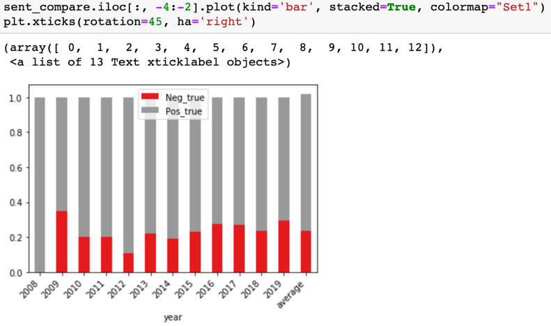
It is quite clear to observe that in the year 2009, and from the year 2016 to 2019, the proportions of negative reviews exceed the historic average which represents in the last bar. This can be further confirmed by:

Insight 2: We have concluded some interesting statistics on Starbucks review sentiments so far, now let's compare us with the rest of the businesses in the city. As a data scientist, it important to not only looking at our own company vertically from different levels but also comparing us horizontally to the industry or to others which operate in the same geographical territory. This is another side benefit to use third party data for analysis, as you get a chance to see how else are doing.
Here is data for the city, and the proportions of negative sentiments are almost 22% and 78% for the positive sentiment.

Furthermore, this dataset provides an attribute called "is_open" which marked the business as either "still open" or "permanently closed". Therefore, another interesting thing we can do is to further divide the data by its status in "is_open". Below is what we got:

What we can conclude from the above table is that:
- (1) We received a higher percentage of negative reviews than the city's overall and all the open businesses in the city, and our review negative rate is closer to the closed businesses in the city. Although there is no direct relationship between negative review rate and business closure, it is worth noticing.
- (2) We have lower positive rates compare to all the open businesses in Toronto.
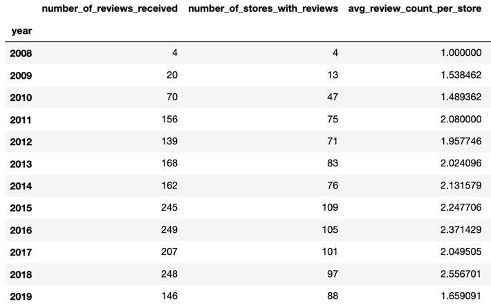
Insight 3: Next, in order to discover more insights from our data, I created a yearly comparison table to include each year's review related information such as "number of reviews received in each year", "number of stores with reviews in each year", and "average number of reviews per store".
Note: the computation steps are skipped and can be found in the original notebook.
This is what we obtain at the end:
Highlights:
If we just look at the most recent year's information at the bottom row which is in the year 2019, there are 146 reviews in total made to 88 stores, and that is less than 2 reviews per store. This is the lowest record since 2011. A year before in 2018, we hit an all-time high with an average of more than 2 reviews per store. This is a warning sign to the business.
Why? Again, I have mentioned that platforms such as Yelp, the actions of leaving reviews are completely voluntary. Usually, for retail chain businesses, customers are more likely to share their experiences for a particular visit when they encounter things (products and services) that are either comparatively better or comparatively worse comparing to the closed competitors or the same retail chain. Nevertheless, having a decent amount of reviews or mentions on social media or any other platforms is a good sign that your brand is still relevant. Yelp is only one source of data, however, for example, if we collect tweets from twitter and reviews from Google and we perform similar analyses and still noticing a drop in mentions or other relevant texts then we might want to dig into the causes.
In summary, as a decision-maker, you want to invest in social media monitoring and it is the quickest and arguably most efficient way to capture your customers' true opinions toward the business.
Let's move on to the store level data
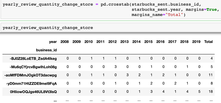
Insight 4: The first thing we can do is to follow up with the last insight regarding the number of reviews over time. We can also create a two-dimensional table that record number of reviews received in each store and each year.
This way, we can help for example the regional manager of Starbucks in Toronto to understand which store draws more reviews in a given year. In addition, if a store receives more reviews in the previous year than a given year. A lot more can be built around this.
Insight 5: Now we are only looking at the recent three years data from 2017 – 2019.
For each year, we can find the store that receives the highest number of positive reviews and the highest number of negative reviews. We can then use this information to help decision-makers to investigate what was going on.
Example: the highest number of positive reviews received by a store in 2019 and 2018 is the same store.

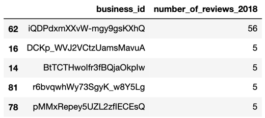
After searching it up using its unique business_id, I found it to be: Starbucks Reserve.

Recall that previously we computed the average number of reviews received by a store in each year and it is 2.6 in 2018, and 1.7 in 2019. For this particular Starbucks Reserve store, it has 47 reviews when it first opened in 2018, and 6 in 2019, both are higher than the average.
From Wikipedia: "Starbucks Reserve is a program by the international coffeehouse chain Starbucks. The program involves the operation of worldwide roasteries; currently six are in operation. Also, part of the program is 43 coffee bars preparing Starbucks Reserve products, what Starbucks considers its rarest and best-quality coffees, usually single-origin coffees." Based on the descriptions, Starbucks is using completely different market positioning strategies for its Reserve bar compared to its regular Starbucks stores. Their products are different and the expectations and experiences thus are different as well. Therefore, depending on the cases, we might want to analyze Starbucks Reserve store independently as it does not represent the general case of Starbucks.
Insight 6: Let's focus on the most recent year's data, we can prepare a table to show proportions of negative and positive reviews received by each store.
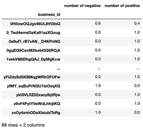
We can even break down the data to months or weeks or even days, therefore we can closely monitor customers' satisfaction over on each store; and with the size of the data, the business can ask someone to look at the specific content of the reviews and intervene as early as possible when customer demand is not fulfilled or in cases when something really bad happened. In the situation of using other data where labels are missing such as Twitter's tweets, we can use our Vader sentiment model or the reviews classifier I will be introducing in a moment to generate the same table.
Insight 7: One last thing to wrap up our "Data Mining & Insights" section is to use a graphical representation method called "WordCloud" to show keywords or terms that are heavily used through all reviews. Note: this is not topic modelling but still very useful for decision-makers to quickly realize important matters that are going on about the business.
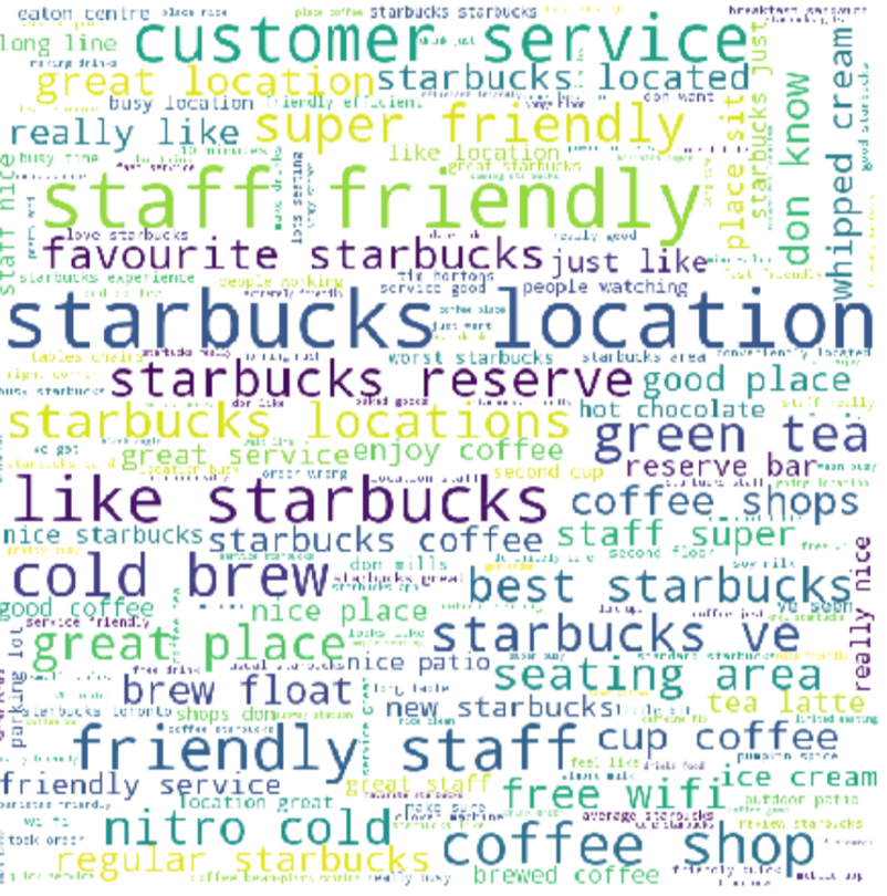
As the font size increases, the importance of the words or terms increases as well.
Part I continue, Machine Learning: building review classification models
Objective: there are two main objectives for this machine learning part
1: Building a classification model that can accurately predict unseen reviews to correct sentiment label class
2: Find out what words are indicative to each sentiment class
Features: I plan to use two different sets of features to build two separate models and compare the results between the two.
Model 1, feature engineering and selection:
(1) Convert DateTime format and extract time-related features from the data:

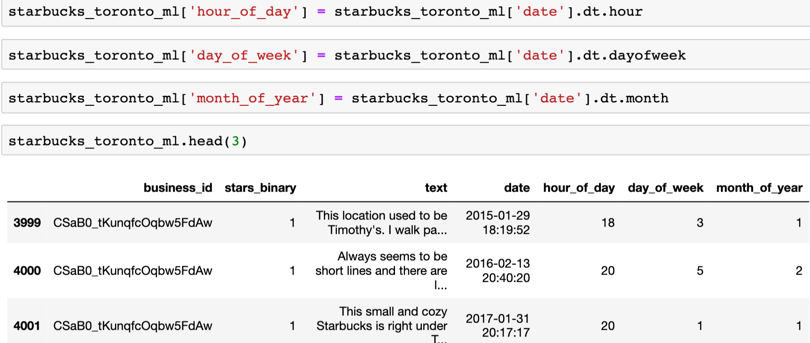
We got new features: "hour of the day", day of the week" and "month of the year".
(2) Extract text-related features:
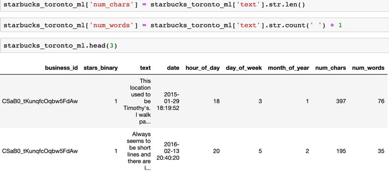
We got new features: "number of characters" and "number of words", and the difference is latter counts for the number of actual words in a text and former includes spaces, punctuations and every other character in a text.
(3) Lastly, I added the result from Vader sentiment model.

Model 1, split the data into training data and testing data
Before we call "train_test_split" module from Scikit-Learn's package, we first examine the distribution of our label class:

As we can see, only 23% of labels belong to the negative class, which means we are dealing with severe imbalanced data.
Recall we did analyses to all businesses in Toronto, and the distribution of negative and positive classes are very similar, and the same applies to Starbucks alone in different years. Hence, we knew that in fact, the distribution of the label classes will remain closer to the dataset we got. Therefore, we must call "Stratify Sampling" technique to ensure the same target distribution is applied to both the training and the testing data.


Model 1, model building and performance measure:
Building the classifier using the Random Forest algorithm and use the cross validation technique to evaluate our result.
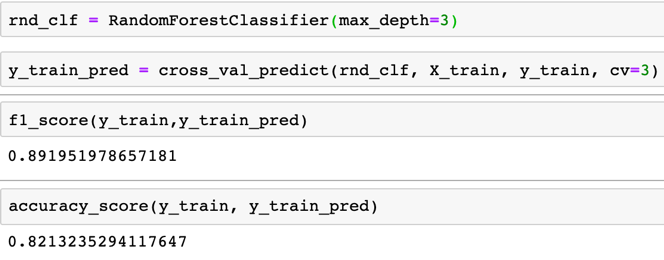
Without searching for optimal hyper-parameters, our basic classifier gives us an accuracy of 82% and with an f1 score of almost 89%. F1 score is the harmonic mean between precision and recall scores. It looks pretty decent, but remember, we have a severe imbalanced dataset, hence our model's ability to predict the minority class is a big question. Based on our use-case, we should care mainly the model's ability to predict negative sentiments. Let's call the classification report to verify the model's true performance.

"0" represents the minority class which is the negative sentiment class in our case. Our model does a decent job predicting the positive sentiments but not the negative sentiments. To give you an example, recall score is calculated as True Positives / (True Positives + False Negatives) and the recall score for the negative sentiment class is 0.36 in our case which means out of all true negative sentiment reviews, the model is only able to predict 36% of them correct. This is not enough.
Model 1, oversampling technique:
To ease the problem with our model's inability to correctly predict the minority class, let's use an oversampling technique called "SMOTE" which creates synthetic instances for the minority class. I introduced "SMOTE" in another project summary called "Employee Analytics Project Demo". For more details about "SMOTE", please visit the official documentation.
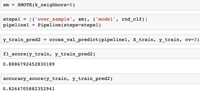
With SMOTE, I created a pipeline object to first over-sample the training data then feed the data to the model. Note, we use cross-validation technique to evaluate model's performance on the training set, and during each fold, a different partition of the training data was over-sampled, but they are evaluated on non-smote validation data.
Now we are getting similar accuracy and f1 score to the previous model, but if we call "classification report", we should be able to see the differences caused by using "SMOTE".
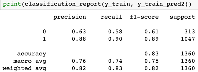
We can see our model's predictive power for the minority class which is negative sentiment has significantly increased, the f1 score jumped from 0.36 to 0.58. We explained recall score before, and now out of all true negative sentiments, our model can predict 58% of them correct. Notice that there was a decrease in the precision score. The precision score is calculated as True Positives / (True Positives + False Positives), which represents out of all predicted to be negative sentiment reviews, the proportions of them being truly negative. The decrease in Precision score means we are getting more false alarms with positive reviews being classified as negative reviews. But this is acceptable, as long as our recall score (ability to pick up the negative sentiment reviews) has gotten better.
Model 1, feature importance:
Let's look at the relative feature importance using this approach:
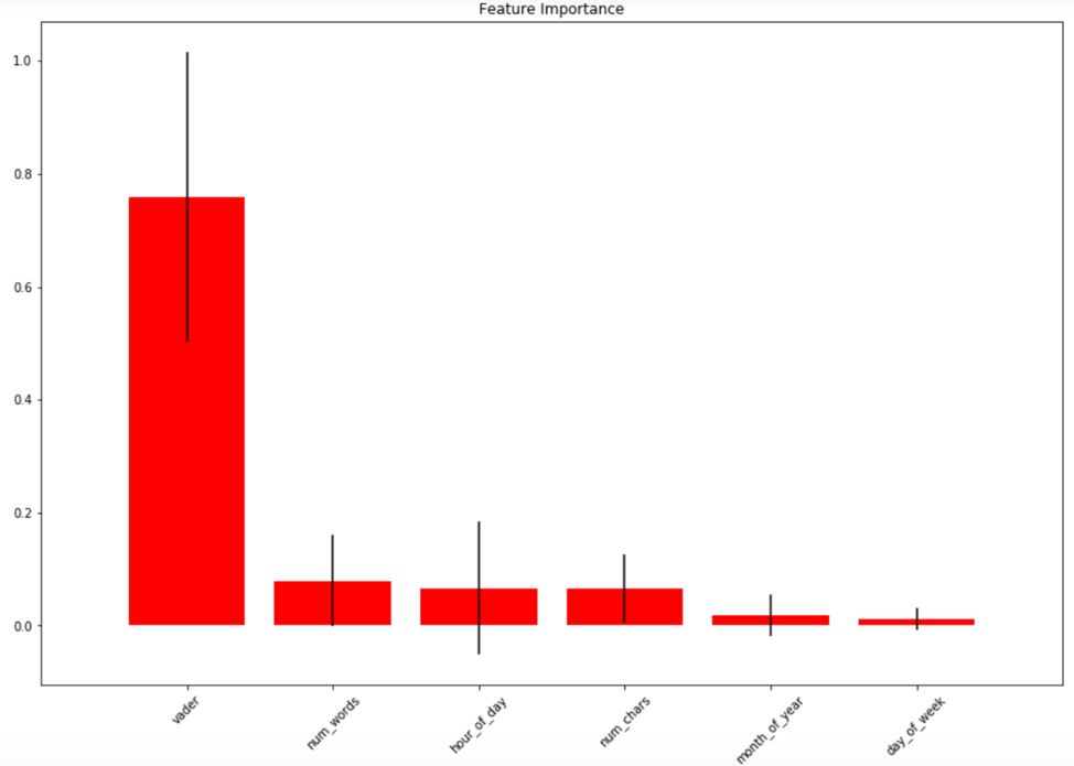
Vader feature plays the most important role to help our random forest model to separate the reviews to positives and negatives.
Model 1, hyperparameter search and prediction on the test.
This part is skipped in this summary, and I have demonstrated how to perform Hyperparameter Search using "GridSearchCV" class from Scikit-Learn in another summary called "Employee Analytics Project Demo". One thing I would like to add is, if we fine-tune our model to fit the training data well, the performance of the model on predicting the test set is likely to be slightly worse.
Model 2, Feature Engineering and Selection2:
Text is an unstructured data type and cannot be utilized on many occasions to build machine learning models directly using algorithms such as Random Forest, Support Vector Machines, Naïve Bayes…etc. However, we can transform text data into its vector representations like numbers, then we can use those algorithms without any problems.
There are different ways to do this, I chose "Bag-of-Word" (short for "BoW") method to transform texts into frequency count of the individual word in the previous "Word Cloud" visualization example. However, instead of using "Bag-of-Word", I introduce a new way to vectorize our text data in this task and it is called "Term Frequency, Inverse Document Frequency" or "TF-IDF" in its short form. This method is widely accepted in the information retrieval and text mining communities and there are different ways to implement this, and I choose the "TfidfVectorizer" class from Scikit-Learn.
If you are interested in the design logic and detailed calculation breakdowns of "TF-IDF", please search the topic in Google, and there are many great articles talk about it in-depth.
Let me briefly explain how "TF-IDF" works, so we can move further in our machine learning life-cycle. Both "BoW" and "TF-IDF" models are designed to help us convert text sentences into their numerical vector representations. The difference is quite obvious if look at the breakdowns of a "TF-IDF" formula. "TF-IDF" is calculated as: "the product of TF and IDF", and the "TF" part is calculated as the same as how you would calculate "BoW" which is by counting the occurrence of a word in a corpus from a vocabulary made up by individual word appeared in that corpus. You can understand "corpus" as a collection of documents or simply as a text dataset. The outcome of the calculation sets the initial relative importance of each word, and the higher the result, the more important a word is.
The second part, inverse document frequency is a way to estimate the "rarity" of a word across all documents. Ideally, we want a word to appear more frequent in one document but not in all documents. If multiple documents contain the same word, the value of IDF will be extremely low such as common stop words in English such as "the", "is", "a". They can appear numerous times in different documents but does not convey any valuable information thus their importance is being "punished".
Wikipedia also provides a high-level summarization of the value of "TF-IDF" which is easy to understand: "The tf–idf value increases proportionally to the number of times a word appears in the document and is offset by the number of documents in the corpus that contain the word, which helps to adjust for the fact that some words appear more frequently in general."
Model 2, moving on to the coding details:
First, I created a new data frame copy and stratify split it into a training set and a testing set (this part is not shown here but available in the notebook). Then I used several text data cleansing techniques to clean the data before I called "TfidfVectorizer" class in Scikit-Learn to help me transform the input data to a matrix of TF-IDF features.
Function to perform wanted data cleaning: the function lowers the string case, remove non-alphanumeric characters, tokenize the data then lemmatizing the words. I will talk more about the use of "Lemmatizer" in the second part of this project.

Feature creation through "TF-IDF":

Note, I included both one-gram, single words and bigram, two adjacent word combinations when transforming the raw reviews.
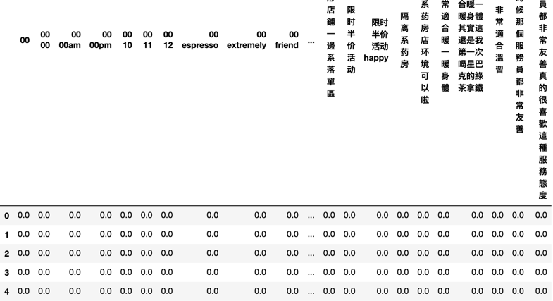
The outcome: the original output for Tfidf Vectorizer is turned into ndarray object and then to a Pandas data frame.
Model 2, building model and performance measure:
Now, it is time to build the model: we are still building a "Random Forest" model, we regularize the model by setting the "n_estimators = 10".

It seems like we are getting a slightly worse result comparing to model 1. If we call the classification report again to evaluate the model's performance in both classes:

We did not use "SMOTE" to help us balance the ratio of negative reviews to positive reviews. As a result of the severe imbalanced class, we can see the model performs very good on the majority class and poorly on the minority class.
Model 2, oversampling:
With "SMOTE", let us skip the implementation details and jump to the classification report:
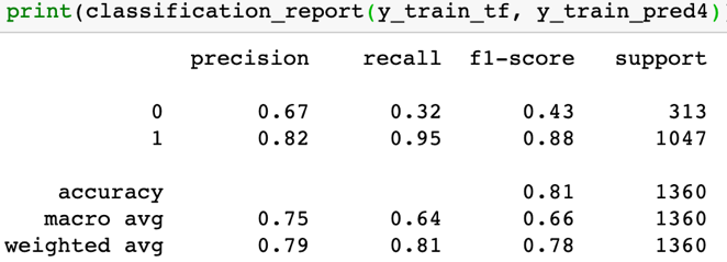
This time, we observe a big increase in our recall score for the minority class but it is not high enough. Comparing with model 1 we previously build we "Vader" sentiments, we would choose model 1 over this since we are more interested in detecting the negative reviews from the business perspective. For future improvements, one thing we should try out is to combine features from both models and see whether that will lead us to a better solution.
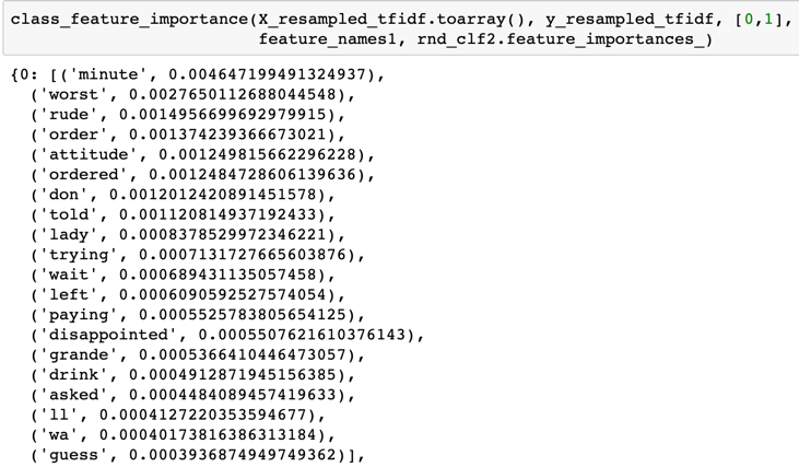
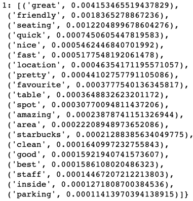
Model 2, finding indicative words:
Find out the indicative words determined by the model to classify reviews to the negative class and the positive class.
First, we can check the words that mostly represent the negative class: in order of importance from high to low
For the positive class:
Model 2, predicting unseen reviews:
The last thing before we wrap up this summary is trying to predict new reviews using our built models.
First, let's create a hypothetical but realistic review example

As a human, we can tell that it is a review with a negative sentiment, although this sentence contains a mix of emotions. How would our model classify this review?
This review must be cleaned and transformed using the same function we used to clean our training data before.
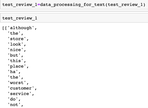
Now, calling our vectorizer object which we used to create TF-IDF matrix:

We can see what our model "thinks" about this review. Is it a positive review or a negative review? We can even access the predicted probability of this review falling into either class.
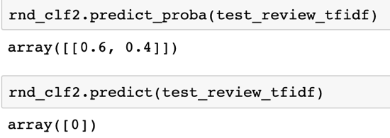
Our model predicts this new review has 60% of chance being a negative review and 40% being a positive review, and it concludes it is a negative review which is correct. For any future reviews, we can do the same thing, clean the data, transform it into TF-IDF representation matrix and calling predict.
Summary:
This is it, the end of the project summary for NLP part 1, "Sentiment analysis on Yelp reviews for a retail chain, the case of Starbucks".
Throughout the work, I demonstrated how to use existing sentiment analysis packages such as "Vader" and "Textblob" to easily discover "hidden" emotions from customer reviews on Yelp. I also explained the importance of leveraging sentiment predictions to help businesses quickly grasp customers true satisfaction and experience towards them. Besides, it is vital for the business to not only focus on internal or vendor data but also investing time in analyzing external data such as those reviews and mentions which spread across various social media platforms as customers are more openly share their thoughts and experiences on those platforms.
