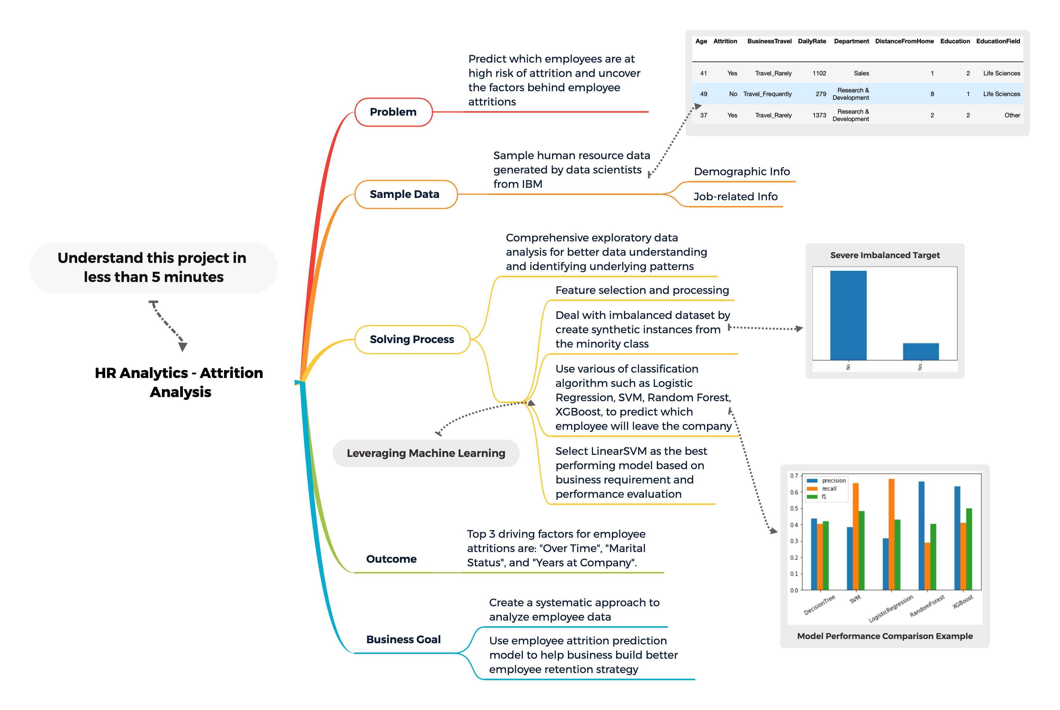
Understand my project in one pic:
Overview:
Human resource analytics, a subdivision of people analytics has garnered significant attention in recent years. In the corporate world, a big part of human resource analytics boils down to improved employee retention. We are living in a fast-paced world with massive media exposure and increasing global connectivity, it becomes somewhat rare that an employee will spend his or her entire career with a single company.
The situation has gotten worse in today's technology industry, with a high reported turnover rate of 13.2%, companies are actively seeking for new solutions to improve workforce engagement and to upgrade existing employee retention strategy.
In 2020, most hiring decisions are still made based on candidate's qualifications on paper, presentations during interviews and each interviewer's own judgement. Thus, a company may hire a star but also one that only shines for a small amount of time.
Using the HR analytics dataset made by IBM data scientists as an example, I created a systematic and statistical approach to analyze human resource data. In addition, by leveraging the power of machine learning, I am able to predict and describe employee attrition. Furthermore, the methodologies used in this project are transferrable and can be applied to any related problems.
Objective:
Identify employee attrition, uncover the factors that drive employee attrition, and ultimately, help companies to improve human retention strategy.
Problem Type:
We want to separate "Attrition" employees from "No Attrition" employees, and we have the target label in our dataset. Therefore, it should be a classification problem.
Methodology:
Tackle the objective with business domain knowledge, data analysis and machine learning.
4 data analysis approaches are covered throughout this project:
Descriptive Analysis: Based on the data available, what relationship we can draw and what patterns we can find.
Diagnostic Analysis : Among all employees who stay or leave, what kind of traits they share in common.
Predictive Analysis : Building predictive models to anticipate which employee will likely to leave the company and the probability of attrition.
Prescriptive Analysis : Based on the predictions, what recommendations we can come up with to help businesses.
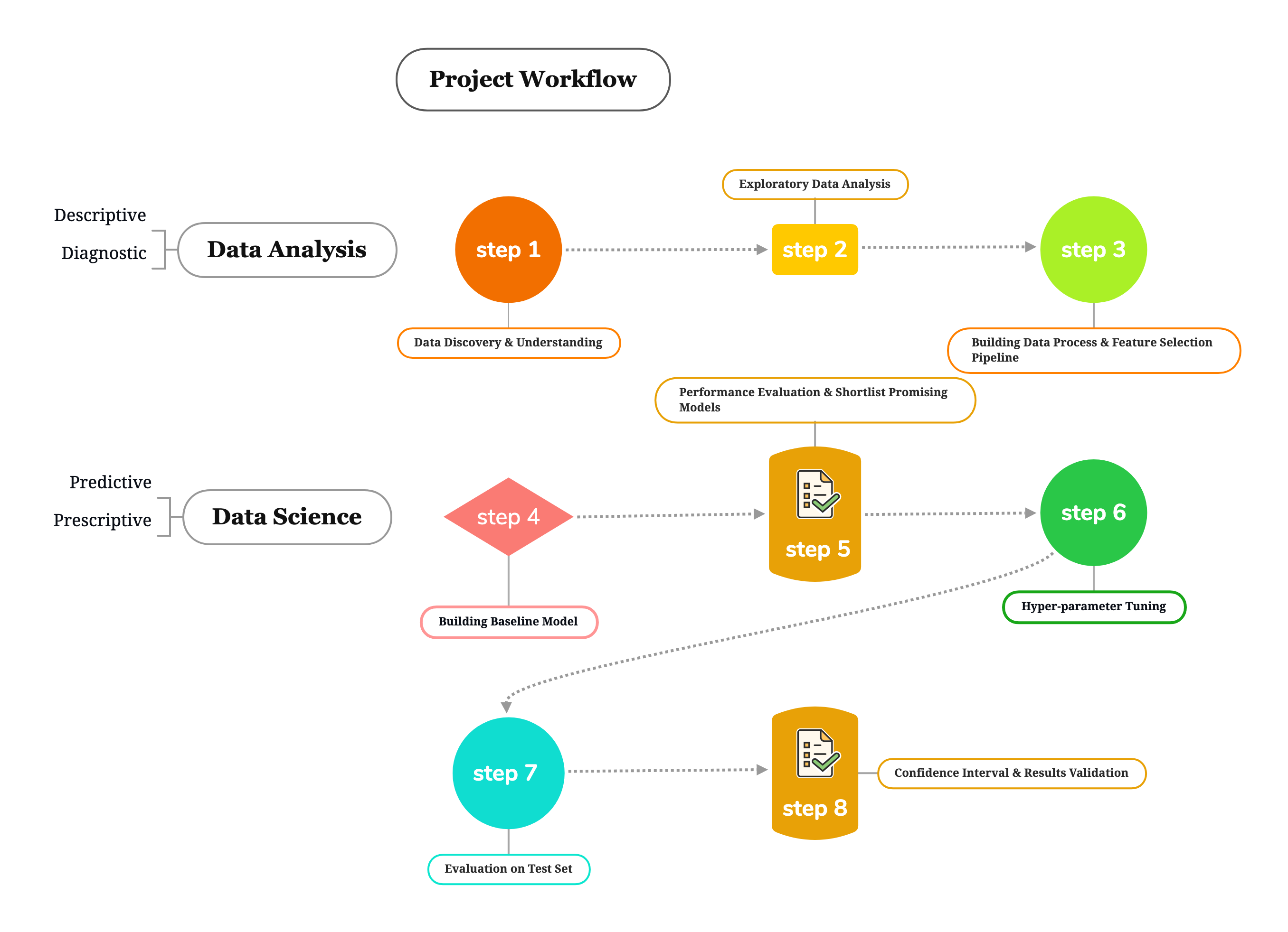
First two analyses are presented in part I "Data Analysis", and latter two analyses are presented in part II "Data Science". Kindly refer to "Project Workflow" for more details.
Data Availability and Selection:
The end goal is to develop analysis approach to Employee Attrition problem. Ideally, we want to be able to solve similar problems with different sets of data.
Representativeness of our data
Real employee data, human resource data are often confidential and protected, so we need to make sure the data we choose is at least representative to the real-world data.
- Does the data contain some key employee metrics that are relevant to us or those that we are currently using? (i.e. "absence rate", "performance index", "employee training expenses"...etc.)
Is the data raw or pre-processed?
In the real world, data has all kinds of incompleteness, especially when it is raw, it has not been standardized, has missing values…etc. When dealing with such data, we need to handle them very carefully, and often time this involves helps from field experts.
For the purpose of this project, I chose "IBM HR Analytics Employee Attrition & Performance" data, and it can be accessed via Kaggle. It is a fictional dataset created by IBM data scientist, and it is clean. Almost all attributes measured are applicable to real-world businesses, and more importantly this dataset has been around for a few years and was used widely by analysts and scientists to study Human Resource Analytics.
Project Workflow
Part I - Data Discovery & Exploratory Data Analysis
Understand the Data
First, we loaded the data into pandas data-frame, and we inspected the data with a shape of 1470 rows and 34 columns. It is not a big dataset but has a decent size of feature space.
Each row represents a unique employee with the corresponding attribute value, and each column is a unique attribute contains either quantitative information or qualitative information about each employee.
Figure 1.1 Gain an understanding of what does the data look like (skipping some features).

Figure 1.2 Complete list of feature names

Quick Data Quality & Fact check
| Check name | Status | Action |
|---|---|---|
| Data Contains Missing Values | No | None |
| Data Contains Duplicated Records | No | None |
| Data Contains Different Unit of Measurement | Yes | Scaling is required |
| Data Contains Columns with Uniformed Values | Yes. "EmployeeCount", "Over18" and "StandardHours" | Drop these columns as they provide no useful information |
| Check Data types | 26 numerical value column and 8 categorical value columns | Encoding the categorical features |
| Timeseries Data | No | None |
After some initial data investigation, we found the data is fairly clean. Some features are not useful for the task and they will be discarded from further analysis.
There are 8 columns with categorical values, and since most classification algorithms cannot take them as input directly, hence we will encode them later.
Understand the label - Severe Imbalance Class
We are working on a classification problem, and we quickly locate our target label "Attrition" from the data. If we zoom in to this feature, we spot an issue of a severely imbalanced class. There are 1233 employees marked as "No" attrition and only 237 marked as "Yes" attrition. Almost 84% of labels are "No".
Figure 1.3 Imbalance Class
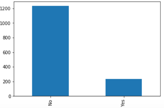
Challenge: the issues come with severe imbalance class are that: 1. it becomes challenge for machine learning models to learn from the minority class; 2. we cannot measure model's performance using "Accuracy", because vast majority of employees would be predicted as "No" attrition, thus ignoring the fact of model's ability to predict "Yes" attrition.
Some common ways to overcome imbalance classes are
- Collect more data
- Consider different model performance metrics (like Recall, Precision…etc.)
- Resample the dataset by either reducing the number of samples from majority class or add copies of samples from minority class.
- Generate Synthetic samples
Solution: The method I chose to use in this project is to generate syntactic samples through a popular algorithm named "Synthetic Minority Over-Sampling Technique", or short for "SMOTE".
Creating a test set
We split the data to a training set and a testing set, and only use the training set for further exploration and analysis to avoid "data snooping bias". The test set is created by stratify sampling the dataset, as a result, the training and the testing set have the same target distribution.

Understand Data Visually and Statistically
Following data visualization/ completion of statistical plots, full visualizations can be found in the Jupyter notebook.
- Numerical feature: histograms, density plot
- Categorical feature: count-plots
- Relationship between numerical features: pair plot, scatter plot
- Relationship between numerical and categorical: box plot and conditional plot
Main findings:
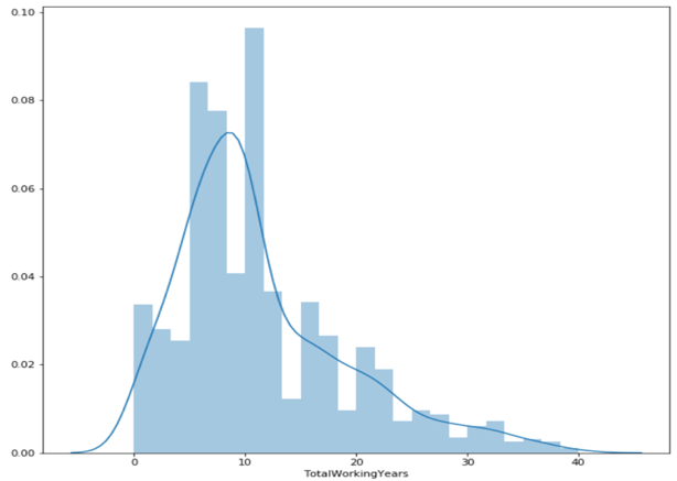
- From histograms, numerical features are presented in different units and range. We know those will create problems for machine learning algorithms to pick up the true patterns from the data. Example: The value range for "TotalWorkingYears" is between 0 to 40 in years, and the value range for "MonthlyIncome" is between 1009 to 19999 dollars.
Solution: use "Standardization" or "Normalization" to treat the data before feeding them to the algorithms.
- Some features are tail-heavy , and they extended much further to the right. Some algorithms prefer to have input data with zero mean and unit variance.
Solution: Combined with the previous issues with data scale, I will be using "StandardScaler" class from Scikit-Learn to treat the data.
Example:
- Many features have outliers in them.
Examples:
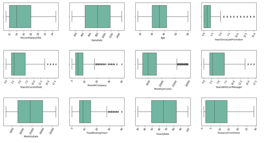
We can clearly spot outliers in features such as "YearsSinceLastPromotion", and "MonthlyIncome". To deal with the outliers, we can either correcting them or removing them.
Solution:But in our case, I decided to keep them as what they are for the following reason:
(When doing people analytics, often you will spot a large disparity among population when comparing certain attributes, and by correcting or removing those outliers will unavoidably increase the bias of the analysis. For example, an average office worker can make somewhere around $55 000 yearly in a company and a Senior VP can make half a million to a million dollars. You cannot just simply remove all Senior VPs from your analysis because the company has less Senior VPs. A better approach can be segmenting the employees to different groups and to analyze and build separate models for different groups. The goal of this project is to distinguish between attrition employees and non-attrition employees and we don't have a large data to deal with therefore keeping them for now.
- Scatter Plot Matrix helps us understand pair wise relationships between two features.
With points (employees) plotted for every two features pair, a few interesting trends can be observed. In addition, I added another dimension, the target "Attrition" to further illustrate the separations of different groups. The findings are:
a. "MonthlyIncome" is a good indicator to separate employees who would leave and who would not, and we will look into this feature later.
b. When "TotalWorkingYears" and "YearsAtCompany" are less than 20, employees are more likely to leave, but when above 20, employees rarely leave.
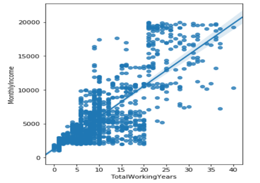
c. Some linear relationships are pretty obvious such as between "YearsAtCompany" and "TotalWorkingYears", between "Age" and "Monthly Income" …etc. These features may be highly correlated which we will examine them later.
Example of linear relationship:
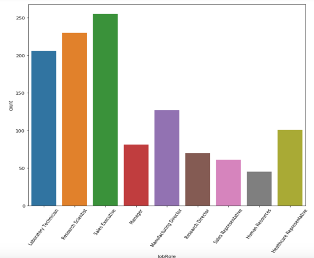
- Through categorical data count-plot, we are able to understand values of each categorical features and understand its distribution.
We need to use the "One-hot" encoding method to encode the data because some features have values that are not ordinal.
Note: some categorical features have a bunch of unique values such as "EducationField"(6) and "JobRoles"(9), when we apply the one-hot encoding method, it will create a number of columns may impact the run time of our model.
Example:
6. Answering Business Questions
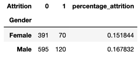
Question 1 : [Gender] We are curious about the attrition behavior among genders. Many studies suggest that well diversified teams with an equal number of women and men perform better in terms of sales and profits, than do male-dominated teams.
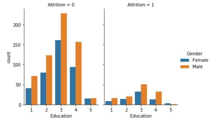
[Education] We are also curious about whether employees educational level plays a role in employee attrition.
Often time, we shortlist candidates based on his or her educational level at early stage of hiring. Thus, we add another dimension which is "Gender" to compare behaviors change with regards to different levels of education.
Answer : 1. Percentages of attrition of female employees are less than their male counterpart. 2. At the highest level of education, level 5, the amount of female employee attrition surpasses male employees.
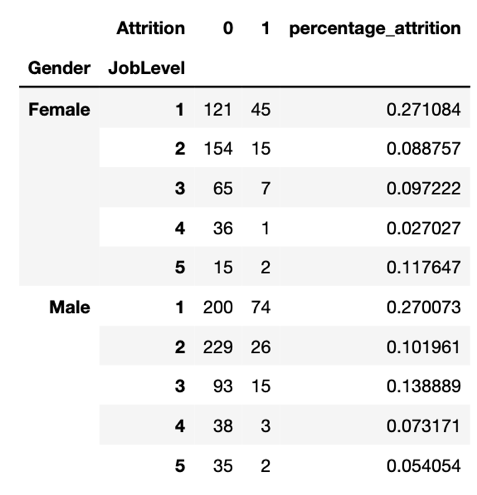
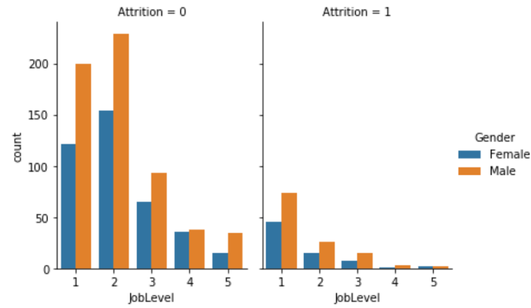
Question 2 : [Job Level] We are interested in finding the behavior changes between females and males at different job levels. It is an important feature to explore, because losing some employees at higher job level can come with greater costs, and it is difficult to find an immediate replacement.
Answer : First, we have a ratio of 40% female employees and 60% male employees. At job level 4, majority of employees who leave are Sales Executives. At job level 5, the amount of female employees that leave surpasses male employees.
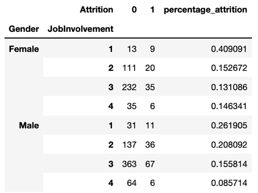
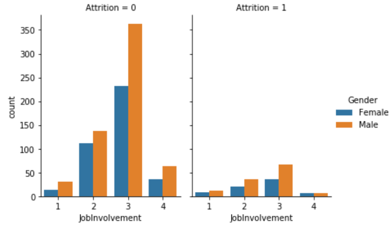
Question 3: [Job Involvement] When we measure employees by their job involvement level, can we spot any interesting trends? This is an important HR metric that companies are known to keep track of. If job involvement is measured by the team managers or peers, can we see some interesting behavior here?
Answer : 1. As job involvement level goes up, generally the attrition goes down, and this applies to both females and males. 2. When employees are at the highest level of involvement at level 4, female employees are more likely to leave.
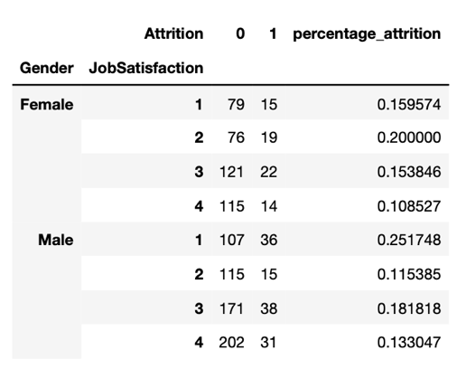
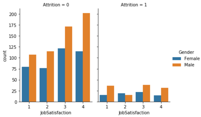
Question 4 : [Job Satisfaction] When taking into consideration of employee self-reported evaluation (like a survey), do we see any interesting trends or patterns? This is from employees' own perspective about their feelings toward their job. Consider this as a quarterly, half-year or yearly survey designed by HR managers to collect employees' satisfaction about their job.
Answer: Female employees are more likely to leave when reported with "Job Satisfaction" equals to 2. More interestingly, female employees with "Job Satisfaction" less than 3 which means less than good, although close, are more likely to leave than their male counterparts. When "Job Satisfaction" is equal to or greater than 3, which means good to excellent, male employees are, although seemingly satisfied, still a lot more likely to leave the company.
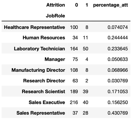
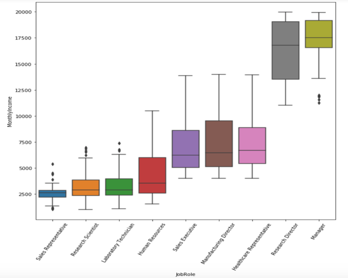
Question 5: Which job role has the highest percentage of attritions from our data? What can be the possible reason(s)?
Answer : (1) The job Sales Representative has the highest percentage of attritions at 43%. (2) The possible reason for high attrition rate may come from its low average monthly income. In addition, a large income gap can be spotted between "Research Director", with smallest percentage of attrition at 3% and "Sales Representative".
More business-related question with answers can be found in the notebook.
7. Identify high correlation variables using Pearson correlation coefficient
We want to identify variables that are high linear correlated. If two variables are so highly correlated they will provide nearly the same information to the model. We don't want to infuse the model with noise.
Linear correlation with our target "Attrition":
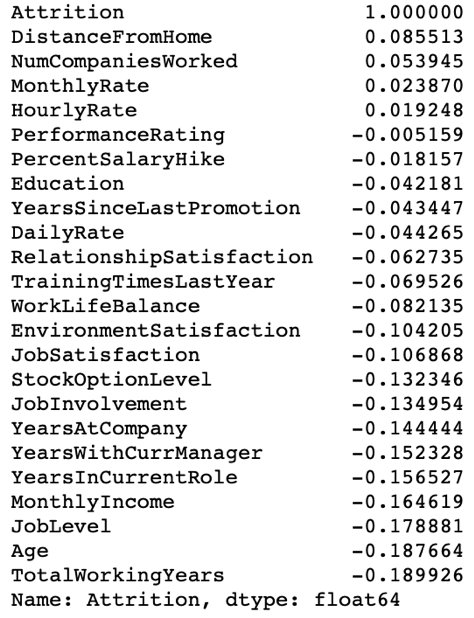
Due to the size of feature space, it is hard to display in this document, and you can find it in the notebook.
We are removing features with correlations higher than 70%, our features to remove are:

Part I Continues - Building Feature Process and Selection Pipeline
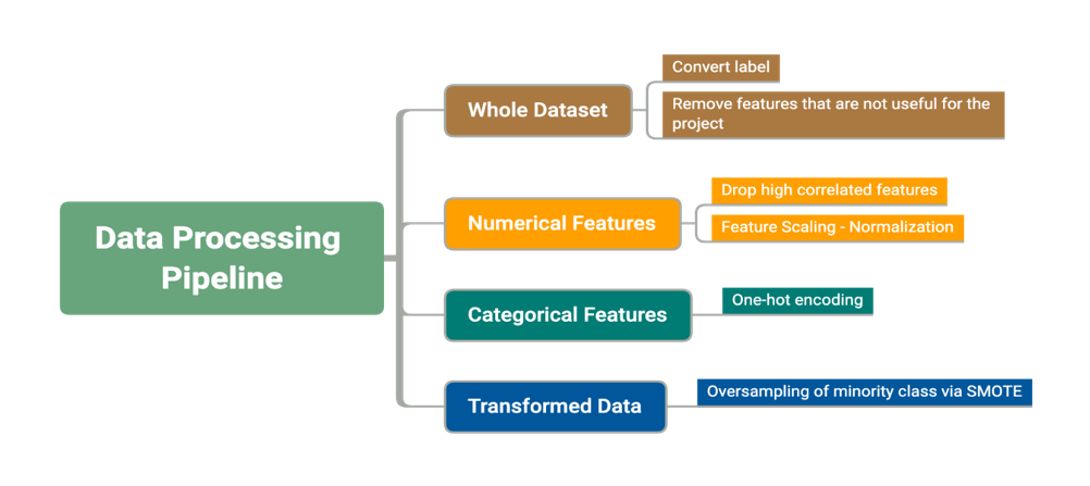
Based on findings from the previous step 1 and step 2:
(1) Convert target labels from "No" and "Yes" to "0" and "1".
(2) Remove features with uniformed value which provide no meaningful information.
(3) Apply standard scaler on all numerical features to ensure they are on the similar scales. This is because I plan to use algorithms such as Support Vector Machine, and by default it assumes all features are centered around 0 and variance in the same order. In addition, since I plan to create synthetic instances for minority class, and I will be using an algorithm called "SMOTE" which under the hood utilizes a KNN (Euclidean distance) algorithm. Thus, scaling is also required.
(4) Drop high linearly correlated features to prevent them from weakening the model
(5) Apply one-hot encoding method to transform text categorical features into one-hot vectors since most machine learning algorithms can only deal with numbers.
(6) Combine above data processing technique to construct a data pipeline and the output of the pipeline is a numpy array.
(7) Use "Synthetic Minority Over-Sampling Technique" short for "SMOTE" to balance the dataset using synthetic samples.
Part II Begins - Building Predictive Models (baseline)
Background:
For the second part of this project, we place ourselves as business owners, and we want to leverage machine learning models to accurately predict which employee(s) are likely to churn. Subsequently, for existing employees, business can utilize proper retention strategy to keep them in place and for hiring new candidate, business can pre-identify high attrition risk employees. Correctly predict whether an employee will churn is our main focus.
Model Selection:
| Model name | Reason to use |
|---|---|
| Decision Tree | Intuitive, easy to interpret, scales to our data even without scaling |
| SVM | Known to handle complex classification problem with small to medium size data |
| Logistic Regression | Easier to implement, and designed for binary classification problem |
| Random Forest | Utilize "bagging" method to reduce variance, reliable feature importance |
| XGBoost | Superior performance, scalable |
Metrics Selection:
Goal: I focus on the model's ability to predict the small positive class (Attrition). Correct detection of employee who would not leave is not my main concern for this project.
Metrics excluded from model performance comparison:
We will not be using "Accuracy" to measure our model's performance since we have severe imbalanced dataset. In this case, models will predict most cases to be the majority class which result a high accuracy score. But our goal is to measure model's ability to predict the minority class.
We will also not be using the "Receiver Operating Characteristics" curve short for "ROC" and the "Area Under Curve" short for "AUC" score to compare our model's performance as they measure performance of both classes by design. With severe imbalanced data set, and our goal for models to predict minority class, they won't provide the information we want.
Metrics selected for model performance comparison:
Recall: recall score is calculated as: TP / (TP + FN), which tells us how many positive attritions we are able to predict using our model.
Precision: precision score is calculated as: TP / (TP + FP), which tells us among all the positive predictions pf attritions, the ratio that we are getting correct.
F1: f1-score is the harmonic mean of precision and recall, it gives more weight to the low value, thus f1-score will only be higher, if both precision and recall are high and with no greater difference.
Model Training
We are still only using the training data at this stage for model training and evaluation, and this is achieved by using cross validation technique.
Example 1: Use pipeline to train decision tree model and use "cross_validation_predict" to get average predictions on the validation data.

Example 2: directly use "cross_validation_score" to access performance metric

Model Performance Comparison:
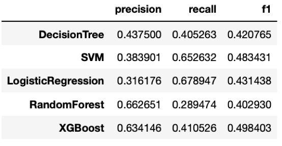
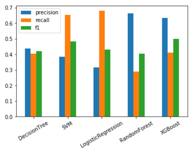
Highlights: 1. XGBoost is the best performing models when we consider both Precision and Recall and close to it is Linear SVM. The differences are, SVM is better with recall while XGboost is better with precision.
- Logistic Regression has the highest recall score compare to others, but when we include precision in the picture, SVM outperforms Logistic Regression
Conclusion : We will be moving forward with "SVM" and "XGBoost".
Comparing performance of "SVM" and "XGBoost" on each class
SVM classification report:

XGBoost classification report:

Highlights : It is obvious that both models perform significantly better with the majority class. Remember we are training the model with sampled data from SMOTE, but when we evaluate our true model performance, we are using the non-SMOTE data.
Note:
Details are not shown here but are included in the notebook.
(1) Precision-Recall curve to show the precision and recall trade-off.
(2) ROC curves and AUC scores
(3) Kernel SVMs
Part II Continues - Hyper-parameter tuning:
Goal:
After shortlisting our models to only two, "SVM" and "XGBoost", now it is time to find optimal hyper-parameters which minimize each model's cost function and also add regularizations to prevent models from over-fitting.
Process:
Searching for the optimal hyperparameter is done using "GridSearchCV" class from Scikit-Learn.
Hyperparameter Selection:
LinearSVM:"C"

KernelSVM:"C", "gamma", "kernel"

XGBoost:"min_child_weight", "gamma", "subsample", "colsample_bytree", and "max_depth".

Again, our goal is to build a model to learn the training data sufficiently and more importantly to predict well on data it has never seen. For detailed explanation and information regarding these parameters, please visit the official documentations.
Hyper-parameter Search Outcome:
LinearSVM: C =0.01
KernelSVM: 3rd degree polynomial with C=0.01, gamma = 0.01
XGBoost: min_child_weight =10, gamma = 1, colsample_bytree=1, max_depth=3
Best Parameter Performance Comparison
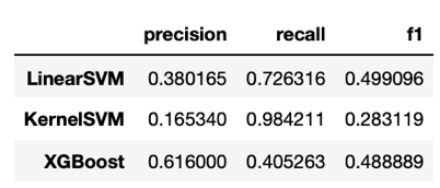
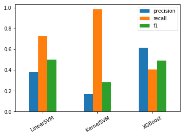
Highlights:
Although it is very close, "LinearSVM" has the best overall performance among predictors in terms of f1.
Although "KernelSVM" achieves supervising high score in recall, on the other hand, its precision score is too low, making the predictions very biased.
Again, "XGBoost" achieves a decent precision score but not doing well with recall.
Final Model Selection:
Final model selection should not be based just on higher performance in numbers but also on fulfilling business requirement(s) and the choice can change over time to accommodate changes in data and demand.
I choose " LinearSVM" to be the final model for this project to measure the generalization error on the test data out of the following reasons:
Based on my experience working in multiple start-up environments,recall is relatively more important than precision in a smaller sized company, as each role is quite unique and the employees usually wear multiple hats and are accountable for a lot of things, therefore finding good replacements can take a long time. As a decision maker, I would rather have a few false alarms than miss any employee that is truly leaving.
However, as a company grows in size thus increasing their budget and decides to use a more aggressive retention strategy to keep the high attrition risk employees, the precision score needs to be high as well. Otherwise, resources are wasted on things that are unnecessary.
In conclusion, the final model selection is based on my assumptions of the business case, and as the famous "No Free Lunch" theorem suggests: if you make absolutely no assumption about the data, then there is no reason to prefer one model over another.
Feature Importance base on Linear SVM
| OverTime_No | 0.596285 |
|---|---|
| OverTime_Yes | 0.509872 |
| MaritalStatus_Single | 0.354313 |
| YearsAtCompany | 0.311033 |
| … | … |
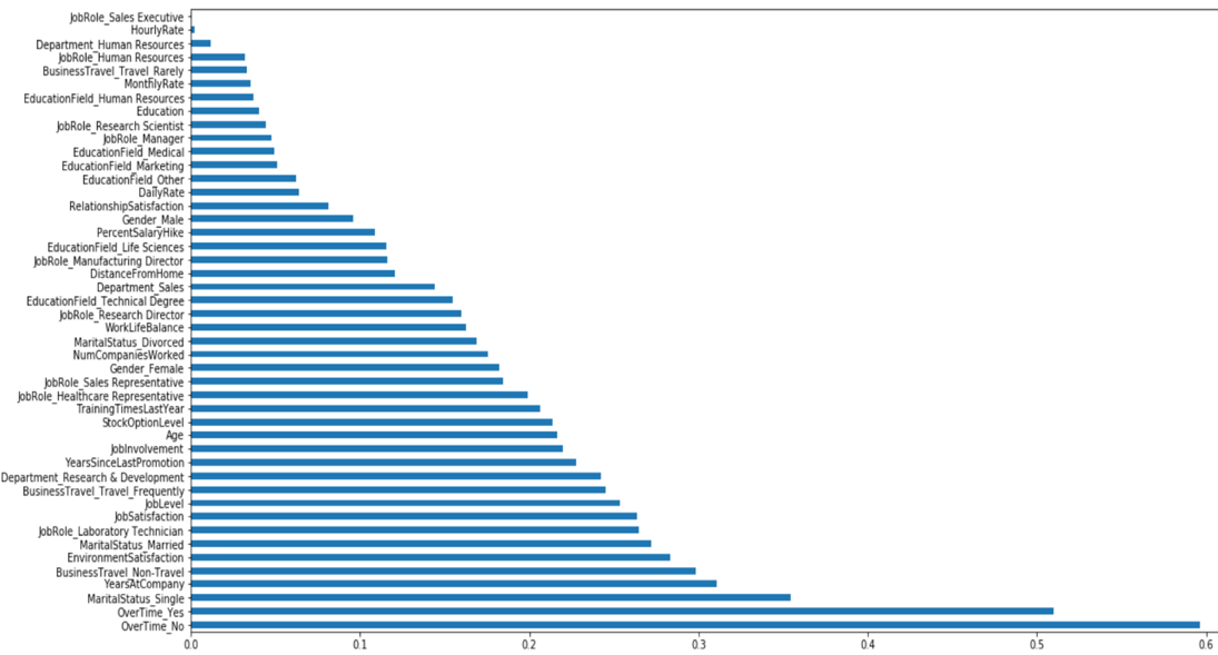
Let's check out top features used by our model to separate our label "Attrition" and "No Attrition".
The records of employee working overtime ("OverTime") are the most important contributing factors used by our model to separate attrition and no attrition class. Another important factor is whether the employee is single or not ("MaritalStatus_Single"). Next is the number of years an employee stays at the current company ("YearsAtCompany"). For complete feature importance, please refer to the bar chart below.
Part II Continues - Evaluation on Test Set
Process:
First, we transform the test data use pre-construct data processing pipeline and then fit the data with Linear SVM of best parameters found from the previous step.
Outcome:

Highlights: the precision score for predicting the minority class which is "Attrition" is 0.39 which is slightly higher that what we achieved using cross-validation on the training data. Noticeably, the recall drops around 8 percent, and the f1-score is roughly the same. The performance drop in recall score can result from us tuning the hyper-parameter to make the model fit the training data well.
Part II – Conclusions
What is this project designed for?
We developed an efficient and effective approach to analyze Human Resource data, specifically to disclose hidden relationships in our data by drawing behaviors of employee attrition from numerous amounts of features available from the data. We built machine learning models to accurately separate attrition group from no-attrition group and it can be used to predict of any employee who will leave or stay in the company given similar data.
Areas of improvement and future works:
First of all, our model is not dynamic by design and cannot predict when will an employee leave the company because we don't have time-series related information in our data.
Additional feature engineering and selections are needed for better performance.
It is worth to try feature extraction technique such as Principal Component Analysis to reduce the feature space.
Lastly, if we are interested in deploying the model to production, we must compute confidence interval of our performance results to gain a more unbiased conclusion.
Part II - Recommendations to the business:
- Sales positions are at high risk of attrition and companies should consider to adopt more active performance measure and utilize progressive retention strategy to keep the high performing employees.
Based on my experience, a static sales compensation plan usually only works for a while, even with some plans that have high reward compensation. In order to keep the employees motivated, decision makers should focus on building inclusive team culture and embed with flexible yet concise reward plans.
Companies should focus on closing the income gaps within the same job role as our analyses indicate employees who leave are those with lower monthly income.
Top 3 factors to determine whether employees will likely to leave their jobs are "OverTime", "MaritalStatus", "YearsAtCompany". Especially, we found that employees who work overtime are high likely to be part of the attrition group. Therefore, employee overtime rather than generating more value for the businesses instead actually costs businesses high price. "MaritalStatus" is important for the model to separate our target groups, but are not so useful in practice as companies don't want to involve any sort of discrimination in hiring and evaluation. If we expand to the 4th and 5th important features, we will also see "BusinessTravel" and "EnvironmentSatisfaction" are also quite useful in predicting employee attritions and all of which should be closely monitored by the businesses.
