This post is the continuation of my previous blog "Post-Campaign Analysis Use-Case Demo Part I".
Recap
In the previous post, I talked about how to evaluate the effectiveness of our marketing offers. I calculated the order uplift and revenue uplift of each offer type and which in turn helped us to find the most effective offer. Furthermore, I built a predictive model to predict the probability of a customer to accept an offer. The model can be used to help the business with revenue forecasting and marketing ROI.
What's Next?
It is time for us to think about do we need to send offers to every customer? Recall that, we divided customers into different value groups using clustering technique, and we designed specific product offers for each group. But, this does not imply that everyone in each group should be getting our offer.
Why not? Because there is the price-insensitive type of customers who are willing to pay the full price. You will lose profit by sending them offers. Besides, some customers will not purchase with or without an offer. You don't want to allocate your marketing resource to them as well.
In conclusion, it is important to figure out a way to analyze individual campaign behaviour and to develop a cost-effective marketing strategy.
Objective
(1) Group customers together based on their campaign response behaviour, (2) Estimate their marketing worth using a combination of machine learning and human set rules.
Work Begins
Data
The data we used is an example of transaction, account and user data from a financial institution. I did a few modifications to make it suitable for our case. Assume this institution wants to target customers for new credit card offers
**Here is what our data looks like:
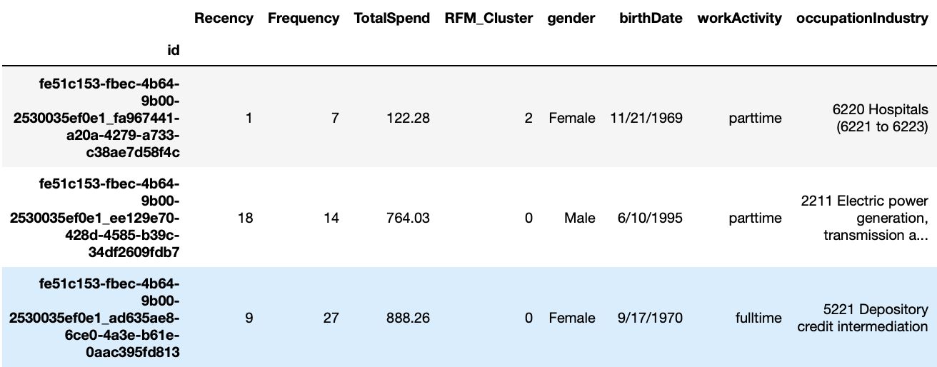
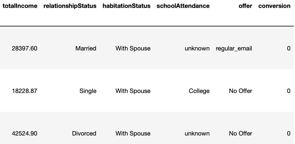
Comparing to the dataset we used in the previous blog, this time we have an additional column called "TotalIncome".
Column Description

Approach
We will create 4 campaign response behaviour categories, and depending on individual customer's response to the previous campaign offers, they will be put into each suitable category. These four categories will be used as our target labels for the machine learning part.
| Group Name | Name Code | Description |
|---|---|---|
| Treatment Responders | TR | A group of customers who accept an offer upon receiving the offer |
| Treatment Non-responders | TN | A group of customers who did not accept an offer upon receiving the offer |
| Control Responders | CR | A group of customers who purchase without receiveing any offer |
| Control Non-responders | CN | A group of customers who did not make a purchase and did not receive any offer |
Target: TR & CN
Based on the set-up from above, we want to target Treatment Responders (TR) because these customers reacted positively to our marketing offers (they accepted the offer). We also want to target Control Non-Responders (CN), although these customers did not make any purchase, they have a chance to be converted once we send them the offers.
On the contrary, we don't want to target Treatment Non-responders (TN) because they did not accept the offer when giving one. Lastly, we don't want to target Control Responders (CR) because they were willing to make a purchase, or in our case, apply for a new credit card without receiving an offer.
Data Wrangling
Step 1: Divide the customers into the "treatment" group and "control" group
customer['campaign_group'] = 'Treatment'
customer.loc[customer['offer']=='No Offer', 'campaign_group'] = 'Control'
This is what we obtain: 82% of customers are in the treatment group and 18% are in the control group.

Step 2: Create a label column
Notice that, we want to estimate the probability of a customer belongs to each campaign response behaviour category. This is a multi-class classification problem.
# Control Non-responders
customer['target_class'] = 0
# Control Responders
customer.loc[(customer['campaign_group']=='Control') & (customer['conversion']>0), 'target_class'] = 1
# Treatment Non-Responders
customer.loc[(customer['campaign_group']=='Treatment') & (customer['conversion']==0), 'target_class'] = 2
# Treatment Responders
customer.loc[(customer['campaign_group']=='Treatment') & (customer['conversion']>0), 'target_class'] = 3
This is what we obtain:

Step 1 and Step 2 combined in one diagram:
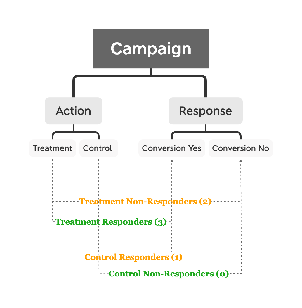
Objective (1) is completed and there are lots of analyses and visualizations can be built on top of this.
Machine Learning
Our goal is to build a multiclass classification model to predict the chances of a customer belong to each campaign response behaviour category.
Feature Selection & Engineering
Step 1: extract customers age from their birthdate
# function to calculate age from birthdate
from datetime import datetime
from datetime import date
def calculate_age(born):
    """this function helps us convert
    customers' birthdate to their age as of today"""
    base_day = date.today()
    return base_day.year - born.year - ((base_day.month, base_day.day) < (born.month, born.day))
date.today()
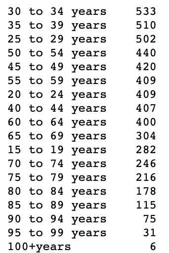
After we apply this function to the "birthDate" columb, we get individual customer's age. Now, we want to group them into different age groups and in 5-year intervals.
bins = [14, 19, 24, 29, 34, 39, 44, 49, 54, 59, 64, 69, 74, 79, 84, 89, 94, 99, 107]
labels = ["15 to 19 years","20 to 24 years","25 to 29 years", "30 to 34 years", "35 to 39 years",
         "40 to 44 years", "45 to 49 years", "50 to 54 years", "55 to 59 years",
         "60 to 64 years", "65 to 69 years", "70 to 74 years", "75 to 79 years", "80 to 84 years", "85 to 89 years",
         "90 to 94 years", "95 to 99 years", "100+years"]
customer['age_group'] = pd.cut(customer['cus_age'], bins= bins, labels = labels, right=True)
This is what we end up getting:
Step 2: Drop unwanted features

Step 3: Encoding categorical features
model = pd.get_dummies(model)
We end up getting 287 columns/features in total. The majority of the incremental columns come from the "occupationIndustry" feaure, as it has 244 unique values.
Modelling
Step 1: Split data into training and testing set
X = model.drop(['target_class'], axis=1)
y = model.target_class
X_train, X_test, y_train, y_test = train_test_split(X,y, test_size=0.2, stratify=y, random_state=42)
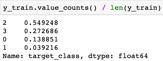
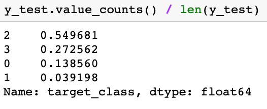
Notice that we set the "stratify" parameter equals to y, hence, the proportion of each category will be similar in both training and testing set.
We can verify this:
Step 2: Building models (For demonstration purpose, only selected steps are shown, full modelling details include hyperparameter tuning available upon request)
#calling an model object
xgb_clf = XGBClassifier()
#learn from the training data
xgb_clf.fit(X_train, y_train)
#predict on the testing data and give access to the predict probability
class_probs = xgb_clf.predict_proba(X_test)
We are calling the model's "predict_proba" to tell us the probability of a customer belongs to each category. An example for the first customer:


Step 3: Use human intelligence to define the rule
We know "TR" and "CN" are our target categories, and the rest two are not wanted. Hence, we obtain the following equation:
The overall target score equals to the sum of the predicted probability of being "TR" and "CN" and subtract the predicted probability of being "TN" and "CR". With this setup, the higher the overall probability, the higher the marketing worth of the customer.
Let's use the example from above, the customer at index 0 has an overall probability of 0.003 (class 0) + 0.96 (class 3) - 0.034 (class 1) - 0.02 (class 2) = 0.927.
Step 4: Let's apply the model and the same calculation method to all customers in the test set
#class probabilities for all customers in the test set
overall_proba = xgb_clf.predict_proba(model.drop(['target_class'],axis=1))
#assign probabilities to 4 different columns
model['proba_CN'] = overall_proba[:,0]
model['proba_CR'] = overall_proba[:,1]
model['proba_TN'] = overall_proba[:,2]
model['proba_TR'] = overall_proba[:,3]
#calculate target score for all customers
model['target_score'] = model.eval('proba_CN + proba_TR - proba_TN - proba_CR')
#assign it back to main dataframe
customer['target_score'] = model['target_score']
Let's take an in-depth look at this new variable by check our its distribution and impact on the target class.
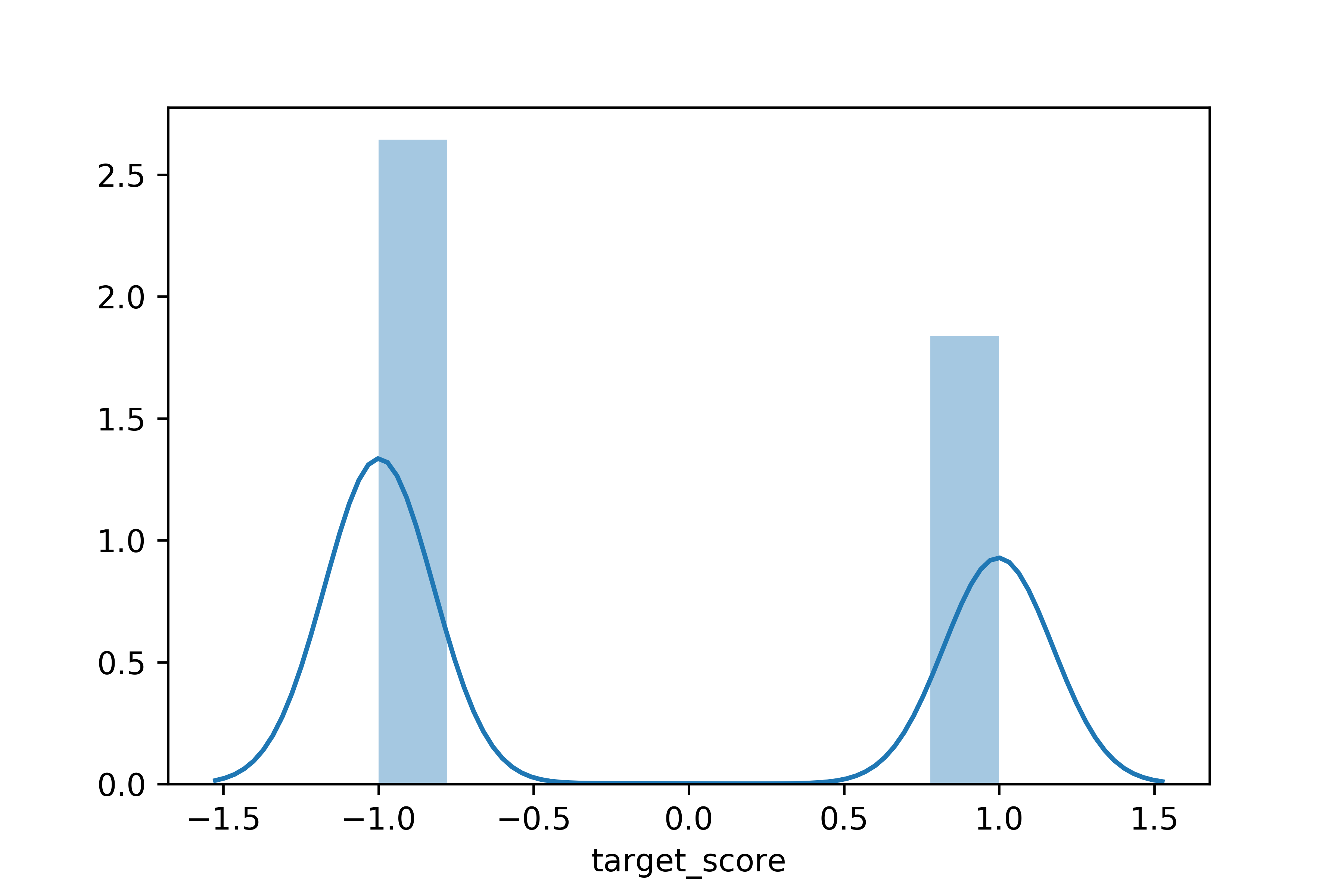
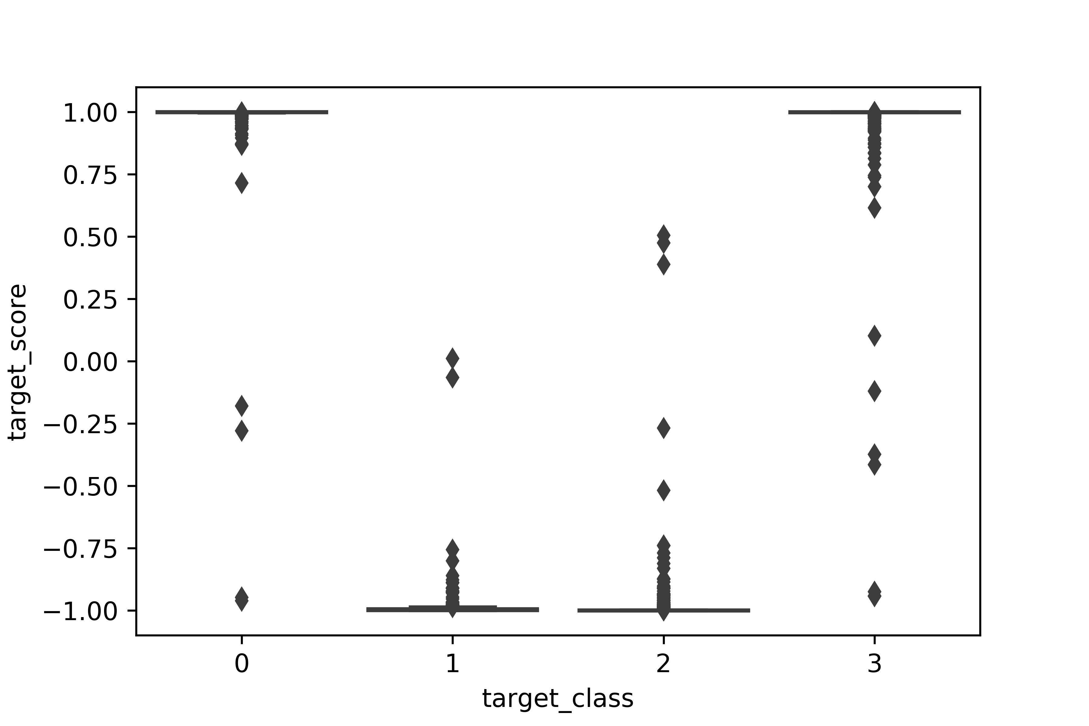
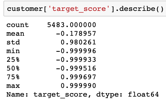
Most of the customers have a "target_score" close to +1 or -1.
Model Evaluation
Now it is time to evaluate the performance of our model. The idea behind the model is to develop an automatic approach to estimate the marketing value of each customer. The higher the overall target score, the higher the customer's marketing value to the business.
By targeting customers with higher overall target score, we increase our conversion rate and saves from costs associated with campaigns.
Step 1
Based on the descriptions above, I proposed to divided our customers to "High Target Score Group" and "Low Target Score Group". The details are shown below:
| Group Name | Description |
|---|---|
| High Target Score | A group of customers with the target score among top 25% |
| Low Target Score | A group of customers with the target score below the median |
Step 2
Now, lets isolate the "High Target Score" group from all customers and for simplicity, we only include "pre-approved" offer type and "No Offer" offer type.
campaign_lift_high = campaign_lift[(campaign_lift.offer != 'regular_email') & (campaign_lift.target_score > lift_q_75)].reset_index(drop=True)
We end up getting 677 customers in total and that is 12.3% of total population:


Notice that, in this group, all conversions come from the "pre-approved" offers, and the "No Offer" group has zero conversion.
Step 3
Next, we borrow the function used in the previous blog to calculate how many incremental orders and revenue boosts are created by comparing customers in this group.
calc_uplift2(campaign_lift_high)
| Name | Results |
|---|---|
| Pre-approved Conversion Uplift | 100% |
| Pre-approved Quantity Uplift | 200.0 |
| Pre-approved Revenue Uplift | $10000.0 |
Let's compare the result with when we included everyone in the target group:

Findings:
- 12.3% of total customers contribute to 10000/11123.309426 = 90% of revenue uplift.
- Revenue uplift per customer is now $10000/677 = $14.77, comparing to the previous 11123.309426/5483 = $2.03.
In comparison, when we look at the "Low Target Score" group, the business will not benefiting from targeting them.
| Name (for Low Target Score) | Results |
|---|---|
| Pre-approved Conversion Uplift | -100% |
| Pre-approved Quantity Uplift | -385.0 |
| Pre-approved Revenue Uplift | $-19250.0 |
Summary
In this post, I demonstrated how to analyze customers based on their campaign response behaviour. I also showed how to build a machine learning model to predict the probability of the customer belongs to each behaviour group. Each behaviour group is viewed as either favourable or unfavourable to the business.
We can leverage this approach and use the predicted outcomes to find the optimal customers to target, and ultimately, optimize the performance of our marketing campaigns.
This series are inspired by author "Barış Karaman" and his "Data Driven Growth with Python" series.
