Understand this project in one pic:
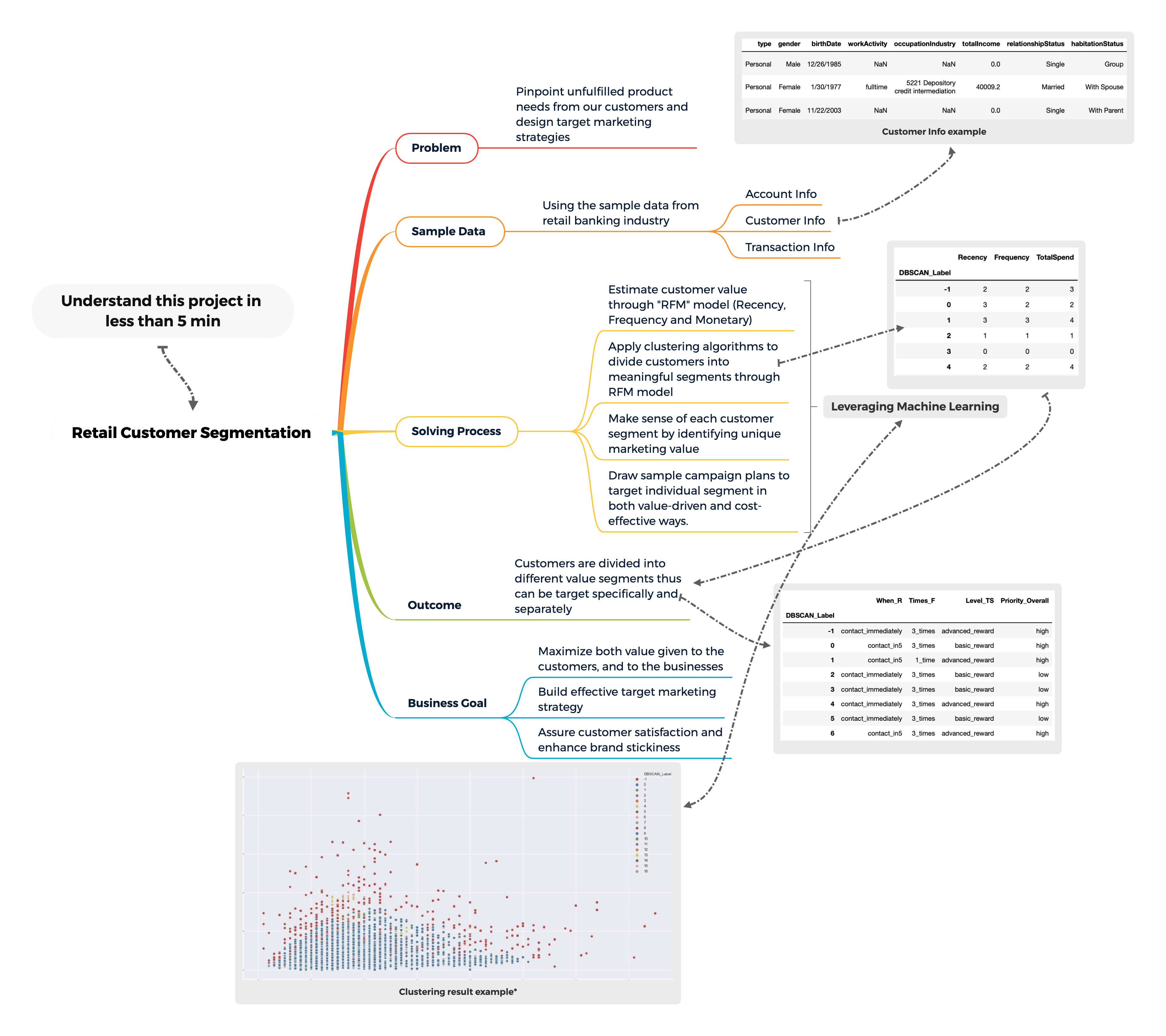
Overview:
In the past 5 to 10 years, retail businesses had shaped their business model to cope with fierce competitions among industry and to adapt to shifts in market demand caused by the technology revolution. Corporations today are competing in big data and analytics-driven world.
If you type "Retail Customer Analytics" in your search engine, in less than half of a second, more than two hundred million results return. If you narrow it down to the "news" section, you will find tons of news about businesses leveraging customer analytics in the real-world applications. Yes, it is no secret that corporations across the globe are using customer analytics to make smarter and scalable decisions. Banks are no exceptions, with millions of funds investing each year in updating modern and sustainable data architectures and building advanced analytics projects.
Why do businesses care so much about customer analytics? If you participate at any investor conferences or take a closer look of their annual report, you will easily spot terms such as "customer-centric", "relationship-focused", and "value-driven", each of which falls to its core mission statement. You will also see terms such as "multi-channel", "omnichannel" in their marketing guidelines.
In summary, businesses long realized that they should not treat all customers the same. All kinds of marketing tactics are in place to ensure customers with diversified value propositions to be completely satisfied. Undoubtedly, businesses want to utilize the power of data mining and analytics to gain a clearer understanding of the value of their customers thus to treat the customers with what they deserve (i.e. through customer lifetime value) via different levels of contact and to intervene before they consider to churn.
Using this project "customer segmentation and analysis in retail banking" as an example, we can quickly separate existing customers to different value groups and help the banks to design effective marketing campaigns to maximize the customer value.
Objective:
We want to apply various clustering technique to segment our potential credit card customers and design suitable marketing tactics for each segment.
Product Assumptions:
In general, commercial banks generate revenues from two big categories: "interest-related income" and "non-interested income". Credit card business contributes value to the banks from both categories. Moreover, based on the report from "Canadian Payment Method and Trend", credit card payment is the second-most-used payment method at point-of-sale in terms of transaction volume and accounted for more point-of-sale transaction value than any other payment methods combined. Canadians love to use their credit cards, according to the same report, nearly 9 out of 10 Canadians have a credit card. Banks and other financial institutions together designed an ecosystem that attracts value to them as early as when customers started applying for a new credit card.
Banks benefit from issuing credit card through the following ways:
At the early stage (non-interest related):
(1) Data harvesting begins when customers use personal information to apply for credit cards and will continue when customers are using their cards for purchases;
(2) Some credit card charges annual fees;
During the lifetime of the credit card
(1) interests through credit card owner's outstanding balance
(2) merchant fees charged as a percentage of the transaction volume or value
(3) cash advanced fees, foreign exchange fees, penalty fees…etc.
Problem Type:
Segmentation using clustering is an unsupervised learning problem since there are no desired labels in our dataset.
Methodology:
The segmentation is based on estimating customer value through a marketing technique called "RFM", which stands for "Recency", "Frequency" and "Monetary". We first transformed our dataset to RFM model dataset and then apply different clustering techniques to segment the customers. The detailed calculations of "RFM" is presented in part 2 of the machine learning section.
Note: although the dataset has no labels, but based on our business domain knowledge, we construct these three attributes with an impression of what the ideal customers look like.
Data Availability:
The dataset was obtained through a job interview data challenge from a local bank and it is the sample of real data with identity and sensitive information removed. It is ideal to demonstrate the data science pipeline from data understanding, goal establishment, data cleaning, data wrangling, building machine learning models and final business implications and analysis.
The original dataset is divided into 3 CSV files, which consists of customer data, account data and transactional level data, and they can be joined together.
Project Workflow
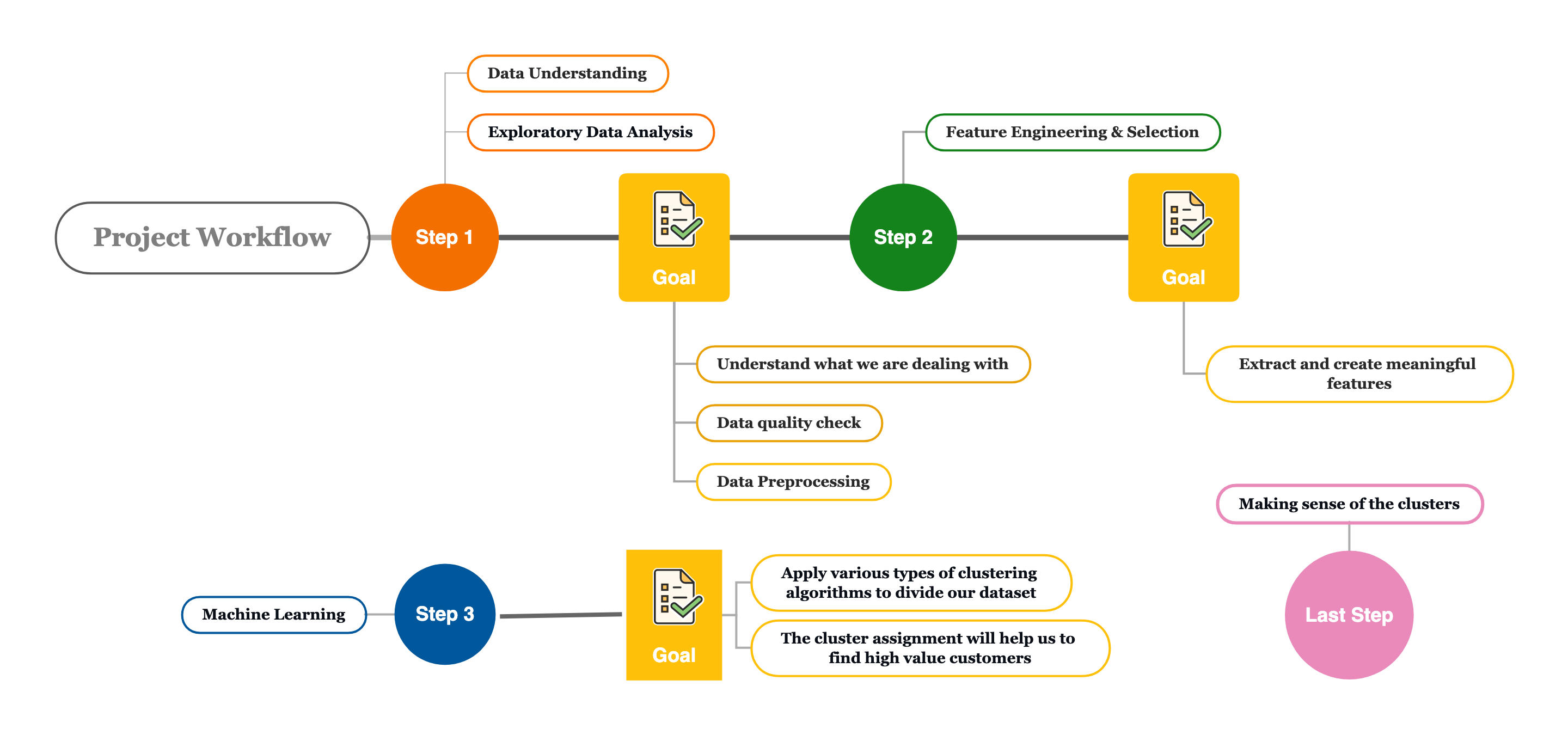
Part I - Data Discovery & Exploratory Data Analysis**
Understand the Data
First, I loaded 3 separate CSV files into pandas dataframe, and I joined the data together one by one using common keys "customerId" and "accountId" separately. I end up getting a new data-frame with 92304 rows and 29 columns.
Each row represents a unique transaction created by a customer, and each column describes the details of that transaction.
Figure 1.1 Gain an understanding of the data look like (skipping some columns).


Figure 1.2 Complete list of feature columns

Quick Data Quality & Fact check
This dataset is raw and not preprocessed.
| Check name | Findings | Action |
|---|---|---|
| Data Contains Missing Values | Yes, 3 columns are empty, 6 columns have portions of missing values | Depends on the further analysis |
| Data Contains Duplicated Records | Yes, all from transaction table | Remove |
| Data Contains Different Unit of Measurement | Yes | Scaling is required |
| Data Contains Columns with the uniformed values | Yes, 5 columns have the uniformed value | Remove, as they provide no information |
| Check Data types | 8 numerical value column and 21 categorical value columns | Keep, at this stage of analysis, we don't need to do anything now |
| Timeseries Data | Yes | Conversions are required |
Data Processing
At this stage, I removed the rows with duplicate records, and columns that are either empty or contain the uniformed value, as a result, I obtained a new data-frame in a shape of 92169 rows and 21 columns.
Here, I also converted "originationDataTime" and "birthDate" from stored "object" data type to "DateTime" data type. Also, I derived each customer's age from their "birthdate".

Now the result looks like:
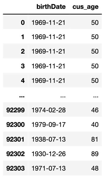
The purpose of having customers' age is for post-segmentation analysis.
- The next thing I did at this stage of data preprocessing is to deal with columns that have missing values.
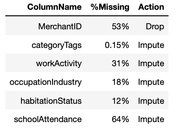
To decide on how to deal with these six are based on the individual analysis result. For example, (a) we simply remove "MerchantID" column, because first of all, percentages missing is a lot. Secondly, each "MerchantID" is coded text and digit combination which cannot be recognized without data dictionary such as the metadata.

(b) I decided to fill in missing values from "categoryTags" with "paydayloan".
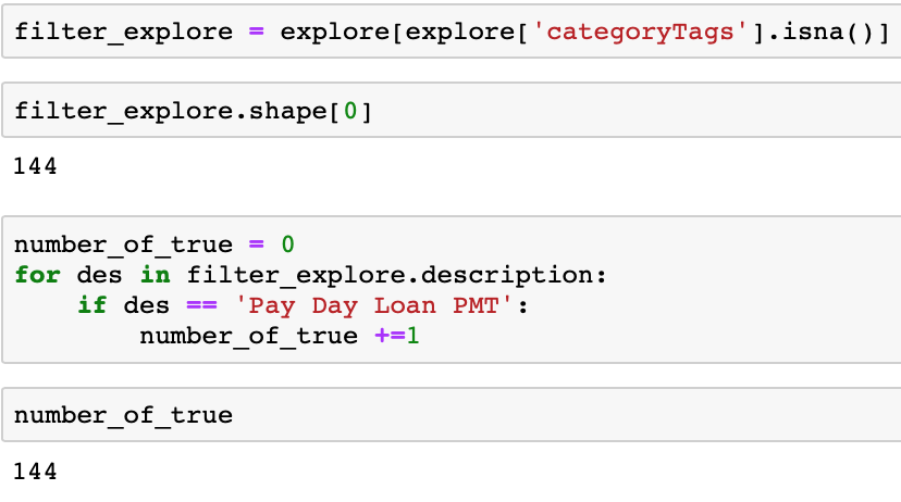
Based on the analysis, I was able to find all records with missing "categoryTags" are identified as "Pay Day Loan PMT" under the table's "description" column.
Rest of the 4 columns are filled in with appropriate values based on the analysis. Again, although we don't include these features now to build clustering models, they become vital afterwards when we decide to compare and analyze the difference among customers between clusters.
- The last thing I did is was to figure out what to do with 5 different id columns, they come from different tables before I merge them. I removed the duplicates and kept only two ids at the end.
Understanding an important feature – "category Tags"
"categoryTags" is one of the most important features for this project, in a sense that our calculation of "Monetary" value will be based on what's included in "categoryTags". Aside from fill in the missing value to "paydayloan", a comprehensive study of what types of transactions are included in each "categoryTags" is completed, and it is mainly based column "description" of each transaction.
| Transfer | contains 'NSF' (no sufficient fund) and "ODP" (overdraft protection fee) |
|---|---|
| Income | contains payroll money |
| Bills and Utilities | contains phone bills, internet bills |
| Food and Dining | contains spending at restaurants and food purchase |
| Taxes | contains: Canada revenue returns and property taxes |
| Mortgage and Rent | contains pre-authorized mortgage and rent payment |
| Shopping | contains spending on shopping |
| Home | contains spending on home decor and others (all from the Canadian tire) |
| Fees and Charges | contains condominium management fees |
| Travel | contains spending on flying tickets |
| Entertainment | contains Amazon Prime membership subscription |
| Auto and Transport | contains spending on public transits and gas |
| Health and Fitness | contains gym membership subscription |
| Kids | contains spending on toys and baby product |
| Payday Loans | contains payday loans |
Understand an important feature – "typeAccount"
There are only two distinct values in "typeAccount" column, "DDA" and "SDA", which is "Demand Deposit Account" and "Special Deposit" account. These can be interpreted as either chequing accounts or saving accounts. All transactions went through either one of these two.
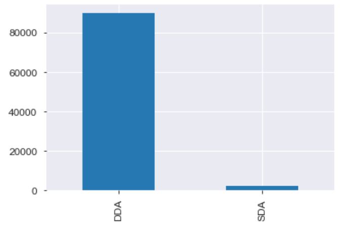
This feature is important in a sense that, it helps me to build the hypotheses to target customers with the "right" products. When we recommend new products to the existing customers, we want to avoid that the products are indeed what they currently owned.
Engineer features for Machine Learning:
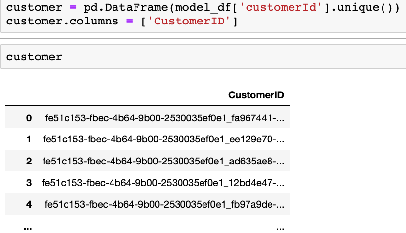
Before we work on calculating values of "RFM", let's create a new dataframe with each distinct customer in every row, and we will be storing the values of RFM and clustering result in this table.
Before we go ahead and create the features, let us first understand the idea behind "RFM" model. The idea is that the most valuable customers are someone who purchased recently, are frequent buyers and spent a lot. On the contrary, the least valuable customers are someone who barely makes any purchases, spends the lowest and purchase a long time ago.
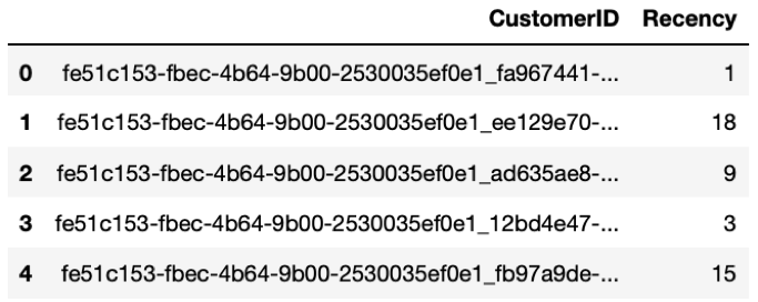
Recency: is calculated by subtracting each customer's most recent transaction date from the most recent transaction date of all customers. We obtain a number indicating how many days the customers have not used their account services. The smaller the number, the better.
This is what we obtained:
Let's look at the distribution (most customers just used our bank account):
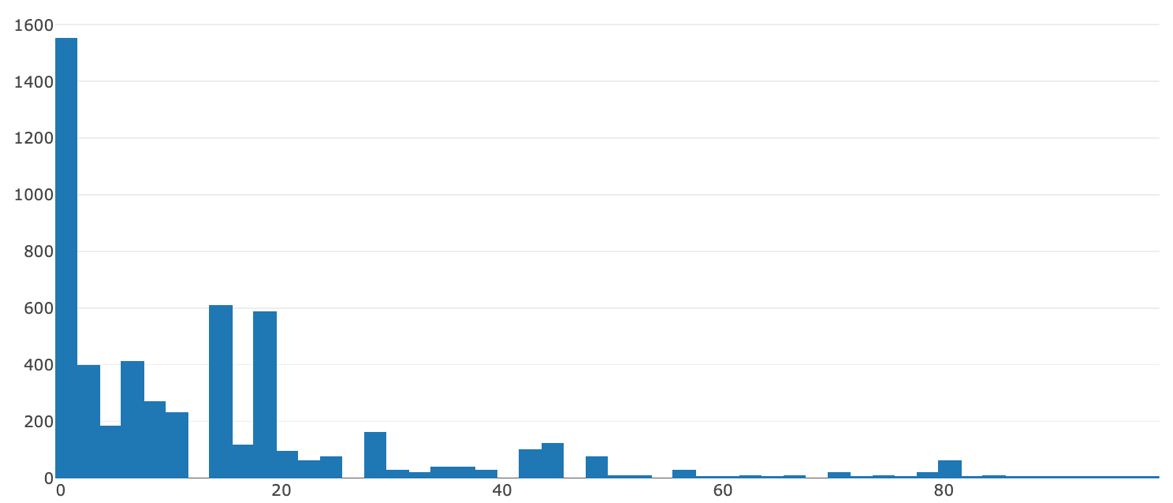
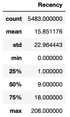
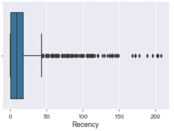
Highlights: There are 5483 distinct customers and the average "Recency" score is 15.8. We can spot a large disparity among the customers because the minimum "Recency" score is 0 and the maximum is 208. This means that the customer with the lowest score, him or her last transaction day is 208 days earlier from the most recent transaction day. The histogram looks far from a bell-shaped distribution; thus, standardization is required for some machine learning models to better learn the underlying patterns of the data. The summary of statistics also shown us the lower, and upper percentile of the data, and I will talk more in later ones.
Frequency: is calculated as the sum all transactions occurred under each individual's account. The bigger the resulting number, the more active each customer is using the accounts.
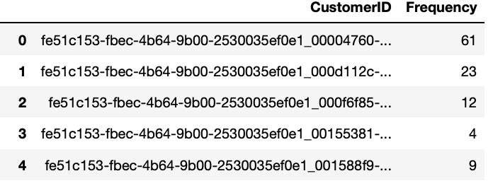
Let's look at the distribution:
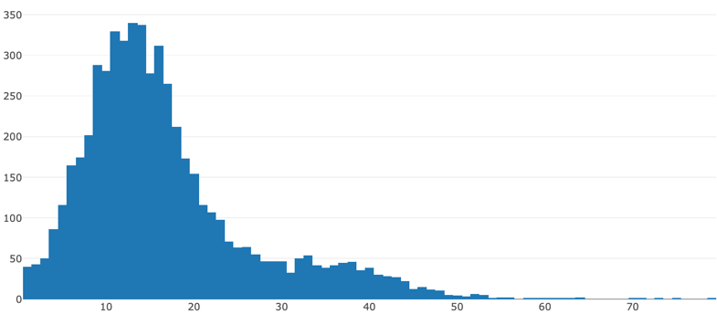
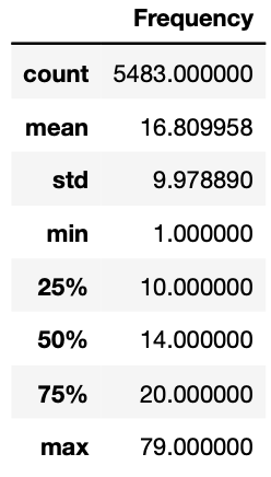
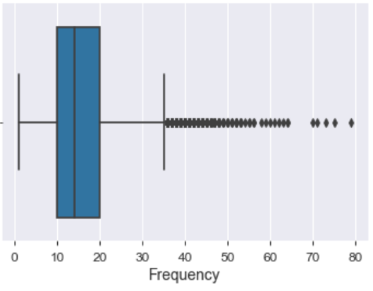
Highlights : based on the distribution plot, it is still tail heavy with more customers above average Frequency value. The 25 percentile indicates that 25% of customers have "Frequency" less than 10, while 50% of customers are lower than 14 and 75% are lower than 20. The "std" or standard deviation tells us how dispersed the data is, and it is smaller than the previous "Recency" value and it is confirmed by looking at the distribution histogram.
Monetary: Recall we want to identify potential customers for credit card offers. Therefore, it is calculated by summing up all the purchases/transactions that can be done using a credit card, and you can look this as calculating the potential spending power of a credit card for each customer.

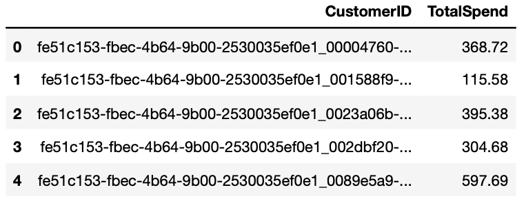
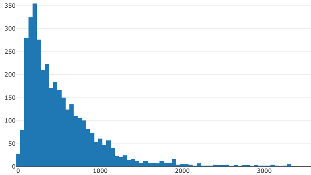
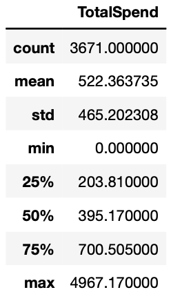
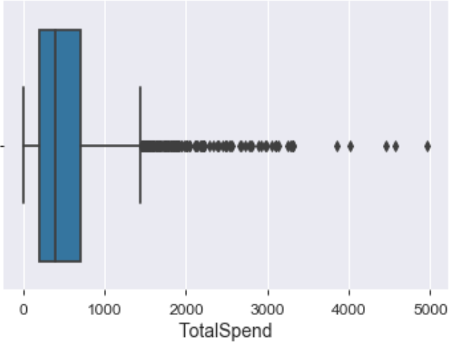
Highlights: there are 1812 (3671 vs 5483) customers with missing data, this means there are no potential credit card transactions under their account. However, we will not be removing them from our clustering analysis because they can be those who bank with multiple banks and primary use others as payment methods. If our cluster analysis categorizes them as high-value customers based on the remaining two dimensions, we can still give them the product offers. Again, proper scaling methods need to be applied due to the skewness of our data.
Data Preparation for Machine Learning
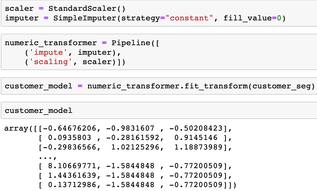
We will first fill in the missing values from "Monetary1" with the number 0, and use Scikit-learn's "StandardScaler" class to scale down features in a way that it will have the properties of the standard normal distribution (curve) with mean =0, and standard deviation =1.
Part II – Machine Learning
Background:
The idea of clustering boils down to separate instances into subgroups with similar traits and assign each subgroup with different cluster labels. For the businesses, we assume customers in the same cluster group share similar product need, thus can be target specifically.
Our goal:
The expectation for this part of the project should be accurately separate customers based on their value derived from RFM methods. The clustering result will be used for downstream analysis.
A brief view of algorithm options:
One major difference to distinguish among clustering algorithms is how "similarity" is measured. Algorithms such as "K-Means" are using centroid based models to group similar instances together, in another word, every instance within the same cluster must have the closest distance to the cluster centroid they belong to than to any other cluster centroid. On the other hand, "DBSCAN" utilizes a density measure to search for areas with high density, it then separates different density regions and assigns the instances in the same density regions to the same cluster. Moreover, I also used a distribution-based model called "Gaussian Mixture", which is a probabilistic model that assumes all the instances within the same cluster are shared with the same Gaussian distribution, and the shape of the cluster is usually an ellipsoid. Lastly, a type of clustering algorithm using connectivity measures that group similar instances to the same cluster when the instances are closed in data space. "Agglomerative clustering" uses the bottom-up approach to connect instances one-by-one and iteratively to create big groups of instances.
Let's check what the data looks like now:
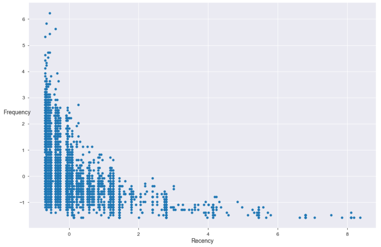
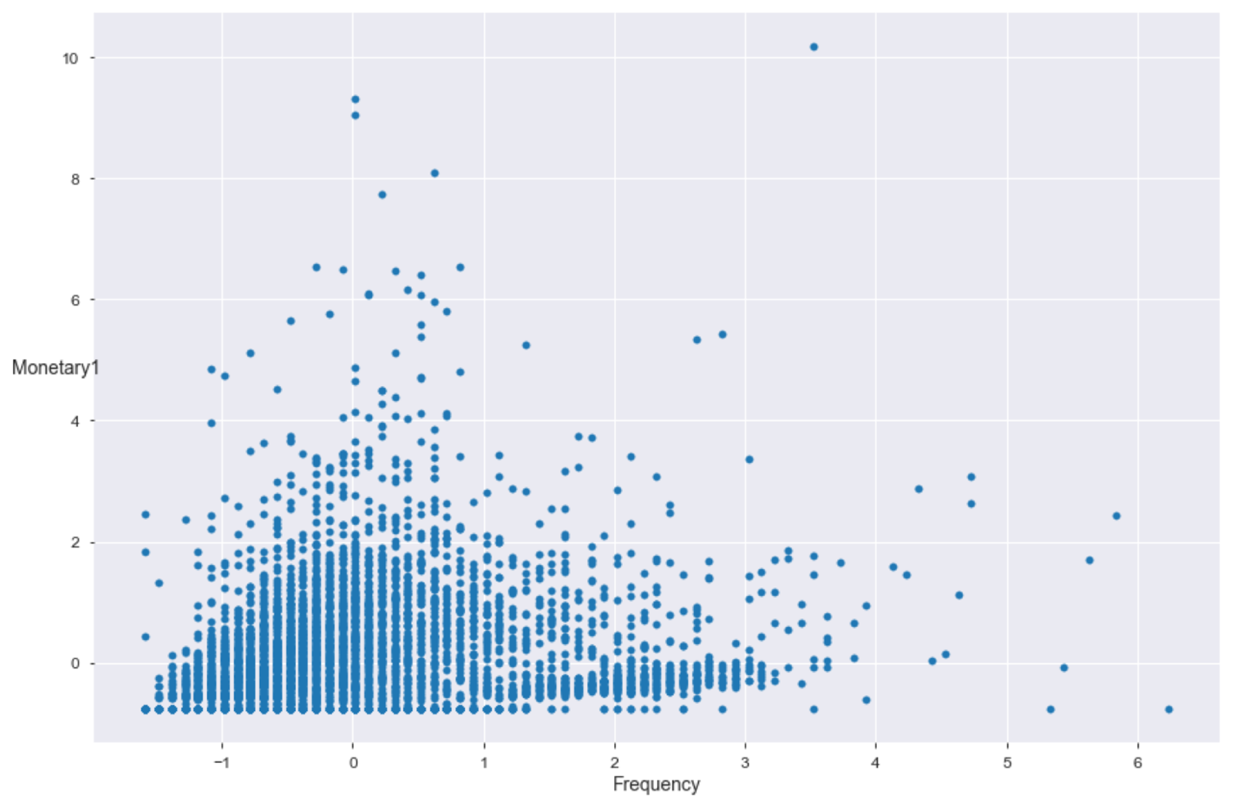
It is important to see where our instances located in different feature space, and this may help us to decide which clustering algorithm to use. Our data has three dimensions, and It is hard to see the data distribution in 3D, so let's plot the data in 2Ds.
We plot the data and hoping to see whether a clear cluster separation can be spotted. Also, based on where the data positioned, it will help us to determine which clustering algorithms to use.
" Recency" against "Frequency"
" Frequency" against "Monetary1"
" Recency" against "Monetary1"
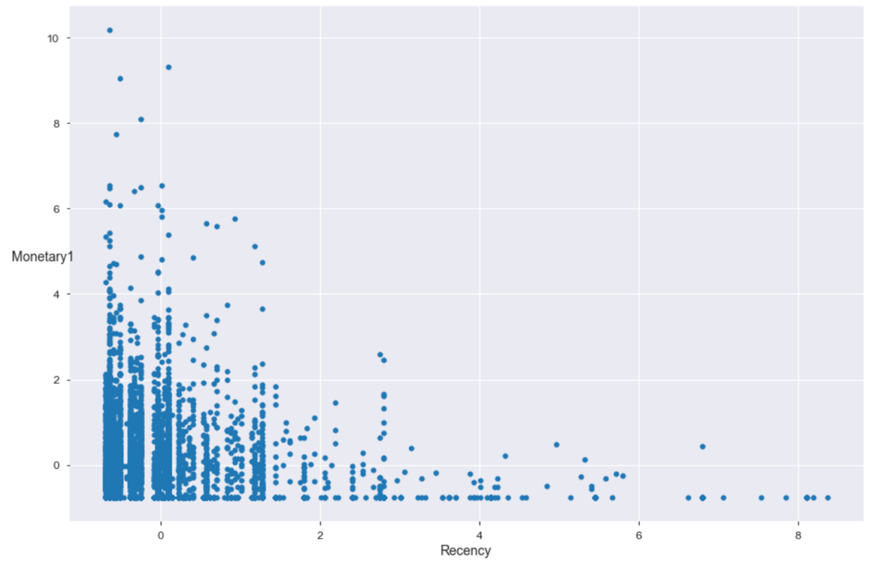
Highlights: (1) It is going to be hard for some algorithms which designed to deal with certain data shapes to perform well. For example, K-Means assumes clusters to have a hyper-spherical shape. (2) We can observe outliers, and use algorithms such as DBSCAN can quickly separate the outliers from the majorities and it is flexible with any cluster shape.
Algorithm Selected
| Names: | Reasons to use: |
|---|---|
| K-Means | Fast and scalable, and guarantee to produce the number of clusters you wish to have. It a special case of GaussianMixture. |
| DBSCAN | Great at separating dataset with various of densities and good at dealing with "outliers". This is important, since the "outliers" can also be higher value customers that are far from an average customer |
| Gaussian Mixture | It can perform "soft" clustering which gives a probability of any instance belongs to each of the clusters |
| Agglomerative Clustering | The size of our data is not huge, and because it's interpretability |
How the number of clusters is determined
| Name: | Ways to determine the number of clusters |
|---|---|
| K-Means | Elbow Method; Silhouette Analysis; |
| DBSCAN | No need to set initial number of k, and it is determined through "eps" and "min_samples" parameters. |
| Gaussian Mixture | Akaike information criterion (AIC) or the Bayesian information criterion (BIC) |
| Agglomerative | Dendogram |
Important Note: different clustering algorithms have different ways to determine the number of clusters and usually by minimizing some performance metrics such as "Inertia" for K-Means.
Cluster number search process & results:
Note: for demonstration purpose, only results from K-Means and DBSCAN are selected and shown, the rest can be found in the notebooks.
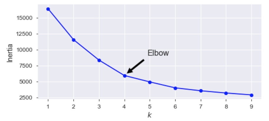
K-Means: both "Elbow method" and "Silhouette Analysis" suggests 4 clusters
Elbow Method: the idea is to find the turning point on the curve where any point before the turning point will result in "Inertia" value to drop drastically and any point past the turning point will have much less of an effect on Inertia value
Silhouette Analysis: the idea is to study the separation result from the cluster model. Silhouette score, in particular, is the mean Silhouette Coefficient over all instances, and we want it to be close to "1" as possible. Because the coefficient of "1" means all instances are well fitted into its assigned clusters and far away from the neighboring clusters.
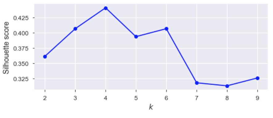
Silhouette Diagram Comparison: it is obtained by plot every instance's silhouette coefficient, sorted by the cluster they are assigned to and by the value of the coefficient. The height indicates the number of instances the cluster contains and the width represents the sorted silhouette coefficients of the instances in the cluster. The vertical dashed line represents the mean Silhouette coefficient.
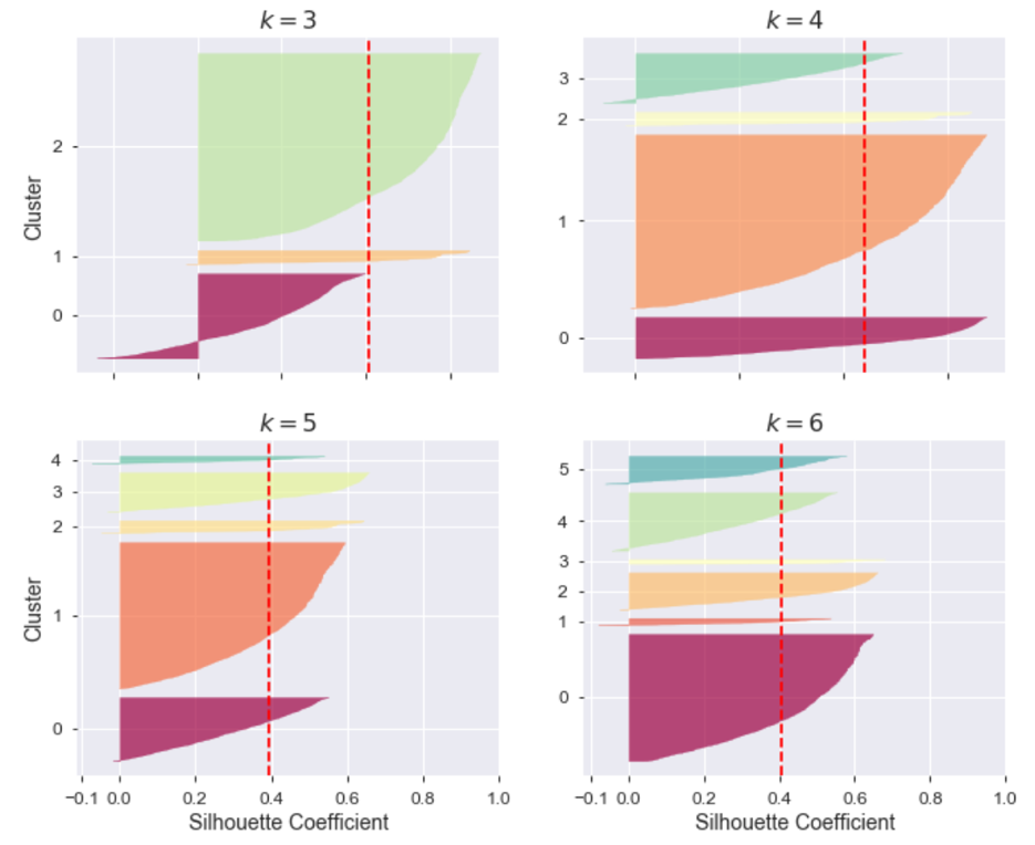
Silhouette score for each possible cluster number:
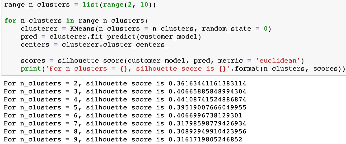
What we have now:
| K-Means | 4 clusters |
|---|---|
| Gaussian Mixture | 18 clusters |
| DBSCAN | NA |
| Agglomerative Clustering | 4 clusters |
Implementation Process:
K-Means:
(1) Decide the number of clusters we want to obtain using silhouette analysis
(2) Select k random points from the data as the temporary centroids;
(3) Assign all the points to the nearest centroid, thus form a new cluster
(4) Calculate the new centroid of each cluster
(5) Repeat from step 3 to step 4 until our clusters do not change anymore meaning all instances within the same cluster remain the same or preset maximum number of iterations are achieved.
DBSCAN:
(1) Finding core instances. If an instance has at least "min_samples" of instances in its pre-defined epsilon distance reach including itself, then it is a core instance. Core instances are always residing in high-density regions.
(2) All instances in the epsilon distance reach of core instances are called neighboring instances and thus belong to the same cluster. There can be multiple core instances in each other's epsilon distance reach, or to say are each other's neighbors, thus the final clusters consist of a long sequence of neighboring core instances.
(3) Any instance that is not a core instance and is not a neighbor of any core instances will be categorized as an anomaly.
Gaussian Mixture:
The assumption for Gaussian Mixture algorithm is that we assume all instances belong to some kind of Gaussian Distribution. Unfortunately, we don't know which instance belongs to which distribution because we don't have the parameter values such as "mean" and "variance" to define a Gaussian Distribution. Therefore, the implementation of the algorithm can be summarized as a search for the optimal parameters that define each Gaussian Mixture distribution or each cluster. The parameter search is done using a technique called "Expectation and Maximization" short for "EM". The idea is similar to what K-Means does to find best centroids but this time, we are searching for more parameter values. The number of clusters is determined by minimizing the value of either AIC or BIC. The EM will run several times until convergence.
Agglomerative Hierarchical Clustering:
(1) It begins with every instance in the dataset is a unique cluster, so if we have 5483 distinct customers in our data, we have 5483 clusters to work on;
(2) At each iteration, the algorithm tries to merge the closest pair of clusters, in another word, merge the most similar customers;
(3) The process will stop once there is only one big cluster left.
Part II - Clustering Results
Note: for demonstration purpose, only results from K-Means and DBSCAN are selected and shown, the rest can be found in the notebooks.
Clustering Result I - Let's look at K-Means first:
We obtain 4 different clusters, and with labels from 0 to 3.
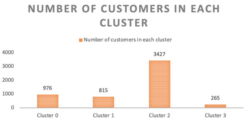
The centroids locations can be assessed by calling "cluster_centers_"

(Let's look at the clustering decisions in two dimensions (i.e. "Frequency" and "Monetary1")
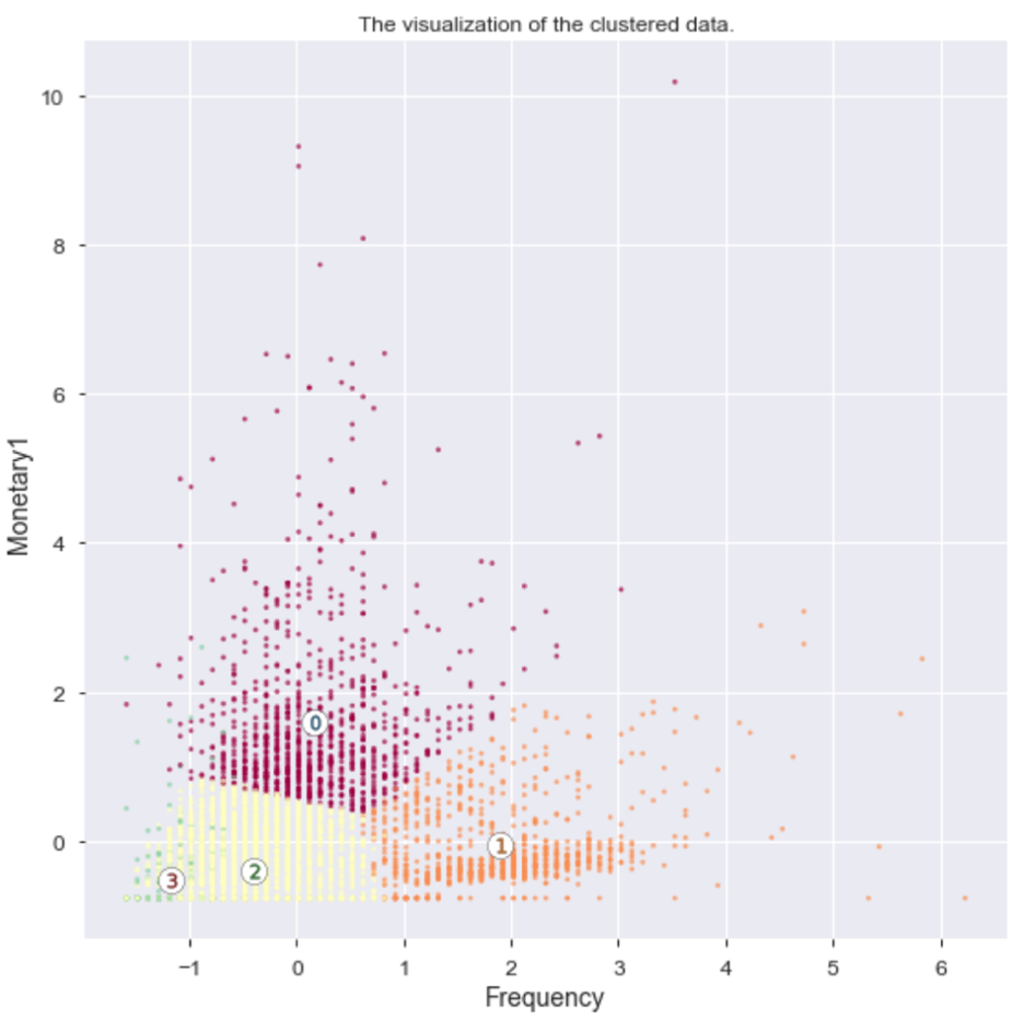
Highlights: we can see lots of overlaps especially on the border regions between cluster 2 and cluster 3.
(4) If we look at the distribution of cluster result for each feature:
Distribution in Recency across all clusters:
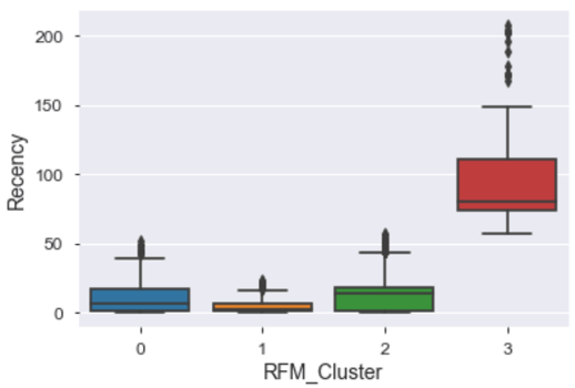
Statistical Findings :Cluster 1 is comparatively short which suggest customers in this cluster overall have low "Recency" score. On the other hand, cluster 3 is comparatively tall, this means customers in this cluster have bigger "Recency" score differences. Cluster 1 also has the lowest median value among all clusters, and we can fairly conclude that cluster 1 is a winner in this dimension.
Distribution of Frequency across all clusters
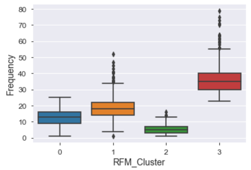
Statistical Findings :unlike "Recency", the score is higher the better for "Frequency". We observe customers in cluster 3 overall have higher "Frequency" than any other 3 clusters. Noticeably, there are quite a lot of outliers from cluster 1 which also have a high-frequency score overall. Cluster 3 won in this dimension.
Distribution in Monetary1 across all clusters:
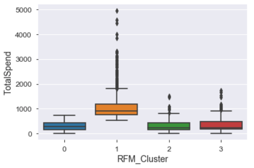
Statistical Findings : it is obvious that cluster 1 has the highest median value among all clusters even with so many outliers. It contains most of the high spending customers and we should target them.
Summary & Business implications: the box plots are used to demonstrate the distributions of customers in each feature dimension across all clusters. If we want to select an overall winner, cluster 1 is preferred in 2 out of 3 dimensions and it was the second-best cluster in the dimension which it does not excel. Therefore, if we were going to use K-Means clustering result to target customers for new credit card offer, we would prioritize customers in cluster 1. An example can be sending them pre-approved credit cards based on their cash flow and credit score.
But this doesn't mean that we will ignore customers in other 3 clusters. Some customers may not have a high "TotalSpend" value as of now, but if you offer them credit cards, you may notice a boost in their spending. Some customers haven't been using our account services for long, such as those in "cluster 3", but according to the "Frequency" feature, they belong to the most frequent user group of our services, thus maybe we should send them reminders, new product offers to wake/activate them.
For customers in cluster 0 and cluster 2, we can also design suitable offers for them although they might not be as active nor as high value as customers in other clusters. However, most of them still have potential spending in using credit cards, we can offer them a low reward type of credit card that doesn't cost the banks a lot.
Another way of thinking: clustering is only the first step
There are several ways to validate the results from our clustering model. For example, in real practice, if we conclude cluster 1 contains the high-value customers we want to target because it achieves an overall high score in RFM models. We can run an additional classification model on top of these customers from cluster 1, and predict whether they are "real" high-value customers against known high-value customers from the past. This way we can measure the true performance of our clustering model.
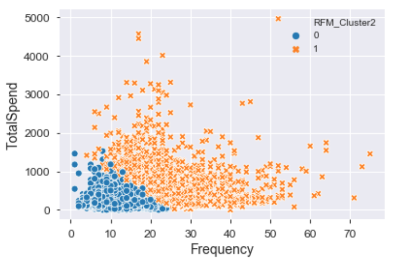
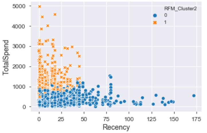
If our assumption changes to only finding high value customers , we can even simplify our model by setting k=2, and this will give us:

The new inertia score is a lot worse than previously with 4 clusters because we force the algorithm to pick only two cluster centroids thus the within-cluster sum of squared distances will be bigger by incorporating farther instances. This clustering result is thus biased but acceptable in certain cases where we have downstream models to perform analysis.

This is the new cluster center locations:

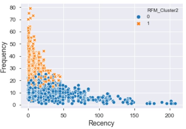
There are only two clusters now, cluster 0 has 3664 customers, while cluster 1 has 1819 customers.

Let's check the boxplots again:
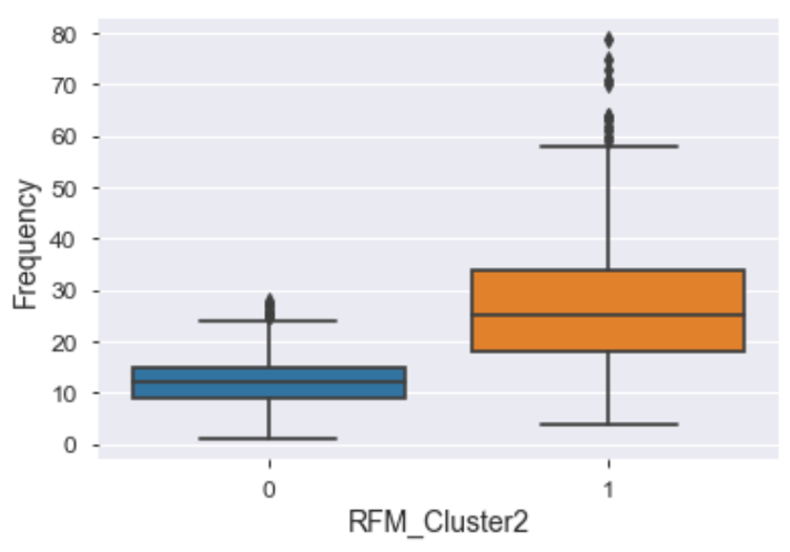
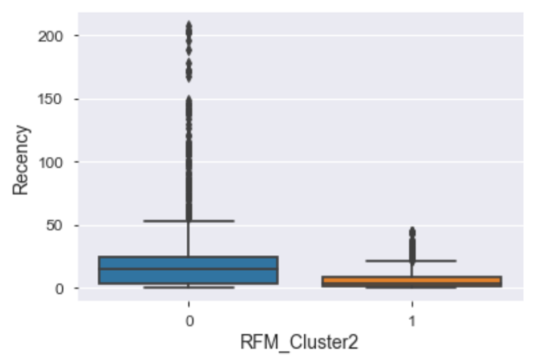
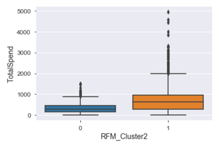
This time it is obvious that we should target customers in cluster 1 because it yields the highest overall RFM value.
We can use scatter plots to show our clustering results:
Clustering Result II – DBSCAN
Decide the optimal value for "eps" and "min_samples"
Before we look at the clustering result, first, recall that DBSCAN doesn't require us to set the initial cluster number (k). It is determined jointly by the parameter "eps" which stands for epsilon distance and "min_samples" which is the number of instances in the epsilon distance.
There is no general rule of thumb to choose the optimal "min_samples", but a low "min_samples" can make the model built more clusters from noise. In our case, we set "min_samples" to be equal to "6", as the original DBSCAN paper suggests that we can set it to be 2 times of our data dimensionality which is 2*3 =6.
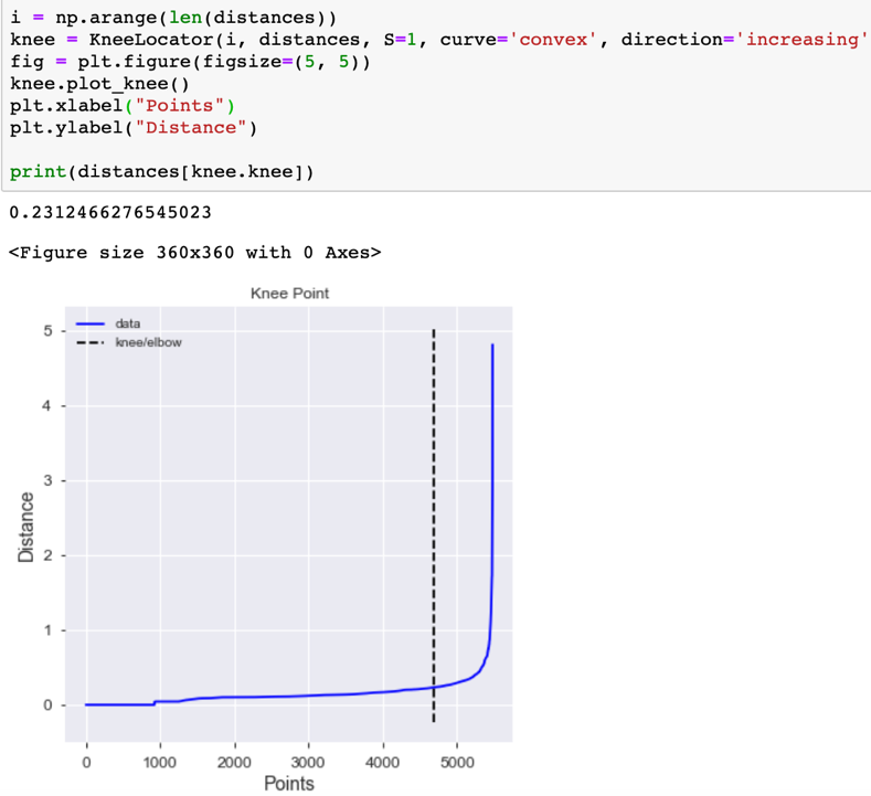
"eps" is determined using "K-Nearest Neighbor" distance plot. The idea is computing the average distances of every instance to its k nearest neighbors. The value of k, in this case, is set to be equal to "min_samples". The k-distance curve is plotted in ascending order and we want to find the "knee" point where a sharp change occurs. Past the knee point, the k-distance curve will drastically go up because this time we are dealing with the outliers which are far away from their neighbors.
We set the "n_neighbors" equals to 7 since the point itself will be considered as the first nearest neighbor, and our knee point is: 0.23
An alternative way to directly show you what cluster decision looks like with different values of k, again we choose only two dimensions as an example.

The plot shown below has a few cutoffs. As the value of "eps" decreases, the number of cluster increases.


Highlights: instances in cluster -1 are considered the anomalies by the algorithm in every subplot, but we will not be treating the anomalies as something completely bad because in our case, although they are far from the majority instances, they represent a group of high-value customers that do not behave like the regular customers. Use the second plot from left in the first row as an example, the majority of anomalies have either the high value on "Frequency" or "TotalSpend" or both.
Final Clustering with the knee point:

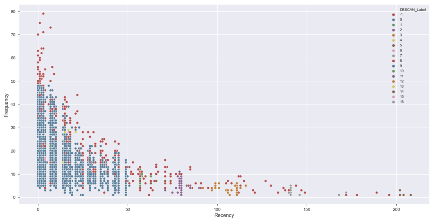
We are getting 18 clusters and one of them is the outlier cluster. Majority of the customers are in cluster 0 which accounts for 88% of total customers.

Let's look at the clustering decision in different feature space:
Recency and Frequency
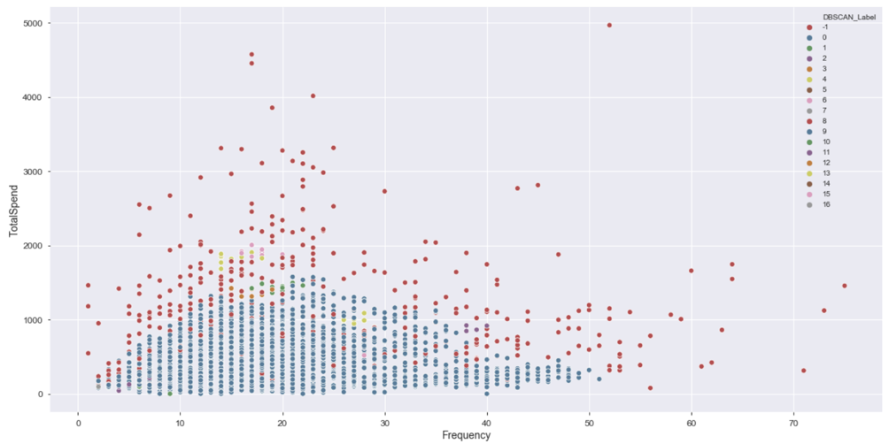
Frequency and Monetary:
Recency and Monetary:
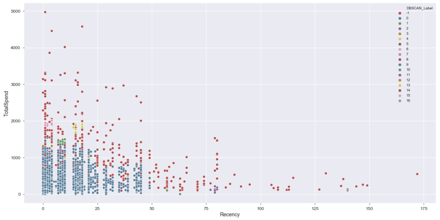
Highlights: Cluster -1, the outlier cluster which is represented in the red dots, contains most of the high-value customers based on RFM estimation and therefore worth most of our attention. This does not mean we should only care about cluster -1 which I will talk about later. Again, using density-based algorithms such as DBSCAN to segment real customer data based on their usage and activity of our products, it acts like a filter that finds extreme points on both ends. We will be picking up all "abnormal" customers, both good and bad.
If we look at cluster distribution in each of three feature space
Recency:
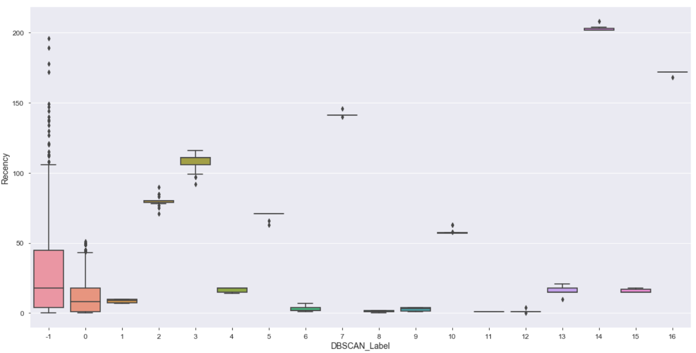
Highlight: In this case, we can easily locate customers that need us to reactivate since they haven't used our bank account service for a long period comparing to other such as those in cluster 7, 14 and 16.
Frequency
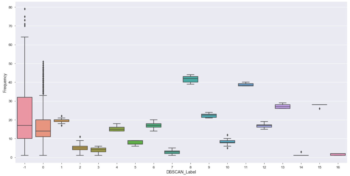
Highlight: there are lots of outliers in both cluster -1 and cluster 0. Outliers located beyond the upper whisker in cluster -1 represent the most frequent user of our bank account services. In addition, cluster -1 has its box shape comparatively taller than any other clusters, this represents a large disparity among customers with various "Frequency" value. Thus, we cannot simply categorize cluster -1 contains the most valuable customers. Further analysis and even additional clustering on top of cluster -1 is required before making any business decision.
Monetary:
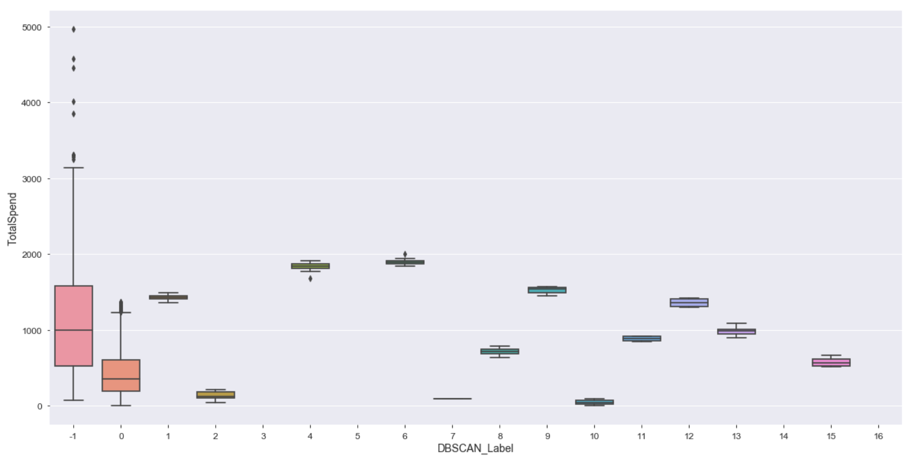
Highlight: aside from having customers who spend the most are considered anomalies in "cluster -1", we can also tell that cluster 1, 4, 6, 9 and 12 have overall high spending customers. Maybe it's worth dividing the clusters into different tiers, thus simply the further analysis.
Issues with having many clusters/segments
Technically we can still study each cluster, and design different marketing strategies for customers in each cluster. However, this will generate greater marketing costs to the business and there are some low-value customers that do not worth the business to invest so much in keeping them activating.
The solutions we propose here is, instead of comparing each cluster with "RFM" value individually. Let's group them into different tiers by transforming "RFM" value to "RFM" rank scores.
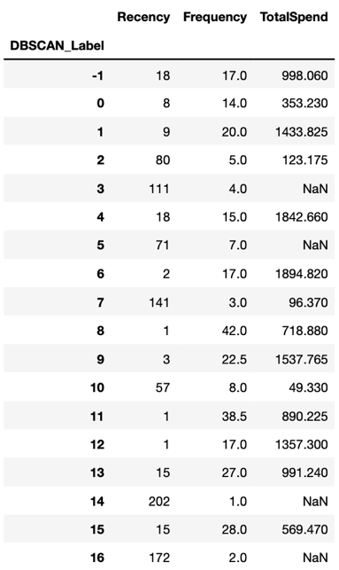
Step one, we group by each cluster, and calculate its median value for each "Recency", "Frequency" and "Monetary". We choose "median" instead of "mean" because we want to generalize the behaviors of each cluster, and some clusters have many outliers that will make big impacts on the "mean" score. We fill in missing values with value 0.
Step two, we use the "qcut" function from pandas to discretize each feature into rank buckets based on its quantiles, and we will get roughly equal-size buckets. Note: we must not forget to reverse the order for "Recency" column since the value is smaller the better instead of bigger the better.
First step: we obtain the following table by group by the clusters, and calculate the median score.
Second step: transform it into "RFM" rank scores
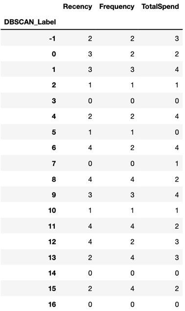
From here, the analysis becomes simpler. The rank scores are from 4 to 0, which represent from the highest value cluster to the lowest value cluster in each feature dimension. We can also give these ranks marketing names such as "Platinum, Gold, Silver…etc.," to describe their relative importance to our business. We can either keep the data this way since each feature suggests a piece of descriptive information which can be directly used to guide marketing strategy. For example, clusters with score "0 – 2" in "Recency" suggest that customers are in low activity level, they need immediate activations. Alternatively, we can aggregate these scores to produce an overall RFM score, and use it to design marketing campaigns. A mixed approach of both is usually preferred.
RFM with an overall rank score: (we simply perform a row-wise sum)
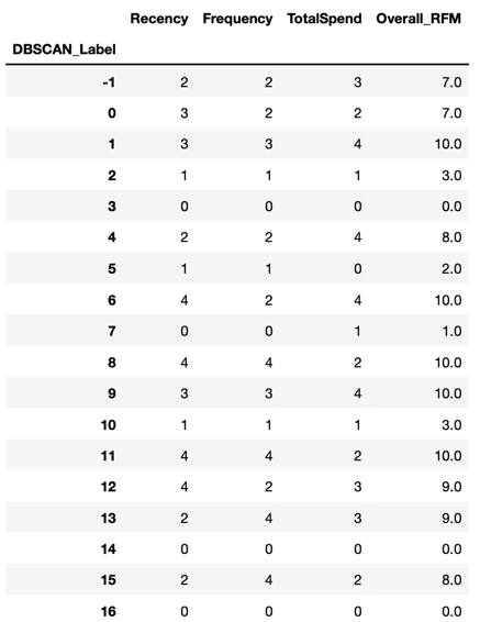
Assumptions: If I am the decision-maker, I would use the "Recency" score to determine how soon we should contact the customers, and use "Frequency" score to determine how often we should contact the customers. I would also use "TotalSpend", also known as "potential spending power in credit card" to determine which level of reward card we should offer and lastly use "Overall_RFM" score to determine the priority level of each customer segment to increase the flexibility of our marketing plans.
In order to bring up some concrete examples, I divided the segments further based on above assumptions, and at the end it looks like: (detailed process is shown in the notebook)
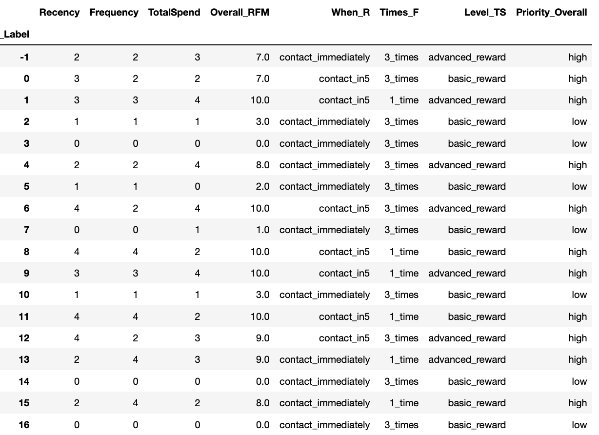
We pick cluster -1 as an example, our marketing team should contact the customers in this cluster immediately with our credit card campaign, and 3 times a week via various contact methods. They should be targeted with our advanced level reward card and they are high priorities.
Of course, the above assumptions build on the hypothesis that those are all the information we own. In practice, we have a lot more to do, such as feeding the clustering result to a credit card default prediction model and filter out high default risk customers. Recall, banks still make money by charging interest from customers' overdue balance but this only works when customers keep using the service by paying at least the minimum amount set by the credit policy. If a customer spends lots of money and disappeared and never pay any outstanding balance then the banks will lose money. Each year, banks could cover up to thousands million dollars in credit losses. A quick way to filter out "bad" customers using our data can be looking for transactions that are either "NSF", or "ODP" as they represent costumers with unhealthy cash flow.
Summary & Business Implications
DBSCAN is a really powerful algorithm to separate the dataset into clusters with various of densities. Depending on the use-cases, sometimes business should not ignore those anomalies set by the algorithm, such as all instances from cluster -1 in our example, as they can represent "hidden" segments that could bring additional revenue stream to the business.
Although the algorithm gives us 18 different clusters, which could be a problem for designing efficient and cost-effective marketing campaigns. The problem can be solved by transforming "RFM" value model to "RFM" rank model and therefore we can break them into different tiers.
Part II – Conclusions
What is this project designed for?
With rising competitions among industry, it becomes insufficient for any business to only understand its customer base altogether at a high level. This project demonstrates how to apply clustering techniques to divide customers into different value segments and by understanding these segments, businesses can build more efficient and effective target marketing strategies.
Moreover, anticipating the unfilled needs of your customer make you a step ahead of the competition as a good product recommendation is a key to increase the revenue and a good product recommendation largely relies on an effective and accurate customer segmentation strategy and planning.
Areas of improvement and future works:
Challenge 1: The way we build our features and the model is rather naïve and in reality, more things need to be considered.
Challenge 2: Although we are using unsupervised learning approach to segment the customers, however, we must have some "labels" in our head or ideas about our target customer. If we know what our ideal customer look like based on historical data, we can turn it into a classification problem to apply further filtering on our data.
Challenge 3: The current approach disregards the path or route that each customer has taken to reach his or her present segment. Segments should be updated regularly over time or when new information comes in.
Future work 1: We need to further analyze our cluster results to see if we can spot any pattern. For example, the distribution of gender, work activity, and age…etc. in each segment. We can also rely on existing customer profiling information to validate the clustering result.
Future work 2: To ensure the quality of our work, we can design ABn testing methods to target those customers and afterwards analyzing campaign response data to compare with the current strategy.
